Comparative Analysis of Different Imputation Methods to Treat Missing Values in Data Mining Environment

(1)

Comparative Analysis of Different Imputation Methods to

Treat Missing Values in Data Mining Environment

Rahul Singhai

IIPS, Devi Ahilya University Indore, India

ABSTRACT

Data cleaning is one of the important step of KDD (Knowledge discovery in database) process. One critical problem in data cleaning is the presence of missing values. Various approaches have proposed to find & replace such missing data including use of mean value, use of global constant, replace by more probable value etc. Imputation is one of the important procedures in statistics that is used to replace the missing values in a data set. One advantage of this approach is that the missing data treatment is independent of the learning algorithms that are used. This allows the user to select the most suitable and appropriate imputation method for each situation. This paper analyze the six different imputation methods proposed in the field of statistics and implement them in Data mining environment. An artificial data set of 1000 records is used to analyze the performance of these methods. For testing the significance of these methods Z-test approach were used. Exhaustive experiments show the effectiveness of the proposed methods. It is assumed that all the attributes of input data are of numeric data type.

Keywords

KDD, Data mining, Imputation methods, Data pre-processing, sampling, attribute missing values.

1. INTRODUCTION

Missing value treatment is another critical issue in data mining. If the information repository on which data mining methods are applied to extract patterns, contains some missing values, then obviously the quality of the pattern extracted may be degraded or poor. Imputation is a promising method used to find & replace the missing values where data set attributes are highly associated to each other. Thus, through the identification of dependency among attributes, missing values can be determined. The objective of this paper is to propose the different imputation methods to improve the quality of KDD process and to compare & analyze the performance of these methods using Z-test in a large database, so that the best possible methods could be proposed in data mining.

2. IMPUTATION METHODS FOR

MISSING DATA TREATMENT USING

AUXILIARY INFORMATION

Several imputation techniques are described by different researchers, some of them are better over others. Rubin (1976) addressed three concepts: MAR (missing at random), OAR (observed at random) and PD (parametric distribution). In what follows MCAR (missing completely at random) is used.

Let



 



N

i i

Y

N

Y

1 1

be the mean of a finite data set under

consideration for estimation. A simple random sample S without replacement (SRSWOR), of size n is drawn from data set







1 ,

2 ,....,

N



to estimate

Y

. The sample S of n units

contains r responding units



r



n



forming a set R and (n – r) non-responding with the sub-space (n – r) having symbol

C

R

in the space. The attribute Y is of main interest and X an auxiliary attribute correlated with Y. For every unit

i



R

, the value

y

_i is observed available. However, for the units

C

R

i



, the

y

_i values are missing and imputed values are to be derived. The ith value

x

_i of auxiliary e is used as a source of imputation for missing data when

i



R

C. This is to assume that for sample S, the data

x

s





x

i

:

i



S



are known and

S



R



R

C. The following figure shows the diagrammatic representation of this sampling procedure.

Under this mentioned setup, some of the well known imputation methods, that can be used in data mining are given below :

2.1 Mean Method of Imputation

(2)













 C r i i

R

i

if

y

R

i

if

y

…(2.1)

Using above, the imputation-based estimator of data set mean

Y

is :



   R i r i

m y y

r

y 1

…(2.2)

2.2 Ratio Method of Imputation

For sampled values yi_andxi_defineyi_as

ˆ













 _C i i i

R

i

if

x

b

R

i

if

y

…(2.3)

where



 



R i i R i i

x

y

b

ˆ

Using above, the imputation-based estimator of data set mean

Y

_is:

RAT S i r n r i S

y

x

y

n

y

_



















 

1

…(2.4)

where



  R i i r y r

y 1 ,







R i i r

x

r

x

1

and







S i i n

x

n

x

1

2.3 Compromised Method of Imputation

Singh and Horn (2000) proposed compromised imputation procedure













ˆ

1 ˆ

1 























 C i i i i

R

i

if

x

b

R

i

if

x

b

y

r

αn

y



…(2.5) where  is a suitably chosen constant, such that the resultant variance of the estimator is minimum. The imputation-based estimator, for this case, is























r n r r COMP

x

y



1 

…(2.6)

Lemma : The bias, m.s.e. and minimum m.s.e. of y_COMP is [As per Singh and Horn (2000)]:

(i) B



y_COMP



=





Y



C

_X

C

_Y

C

_X



n

r

















 



1

2

1

…(2.7)

(ii) : M



y_COMP



=

1

1 Y

2

C

_Y2

N

r











 











C

X

C

Y

C

X



Y

n

r





















 



1

2

1

2 2

2

1

…(2.8)

(iii) : For optimum

















X Y

C





1

, the minimum m. s. e. of yCOMP is given by the expression



y

COMP



min

M

= 1 1 1 1 2 S_Y2

n r N

r _

                  



…(2.9)

2.4 Ahmed Methods of Imputation

For the case where

y

jidenotes the ith available observation for the jth imputation method. Ahmed et al. (2006) suggested the following:

(A):



1



1 1                            _C r n r i i R i if y r x X y n r n R i if y y  …(2.10)

Under this, the point estimator of

Y

is

1 1           n r x X y

t …(2.11)

Lemma :

(i) The bias of t₁ is :

 



_











_











 



Y

C

_x

C

_Y

C

_X

N

n

t

B

₁



1



1 2



₁



2

1

…(2.12)

(ii) The m.s.e. of t₁ is :

 

                            

 Y x CYCX

N n C N n C N r Y t

M  1

2 2 1 2 2 1 2 1 1 1 1 1 1 …(2.13)

(iii) The minimum m.s.e. of t₁ is :

 

2 2₂

(3)

for the optimum value of



₁ which is given by X Y

C



 

1 .

(B)



1



2 2                          _C r r n r i i R i if y r x x y n r n R i if y y  …(2.15)

Under this, the point estimator of

Y

is

2 2 















r n r

x

y

t

…(2.16)

Lemma

(iv) The bias of t₂ is :

 



_











_











 



Y

C

_x

C

_Y

C

_X

n

r

t

B

₂



2



2 2



₂



2

1

…(2.17)

(v) The M.S.E. of t₂ is :

 

_                            

 Y x CYCX

n r C n r C N r Y t

M



2



2 2 2 2 2 2 2 1 1 1 1 1 1 …(2.18)

(vi) The minimum m.s.e. of t₂ is :

 

2 2₂

min 2

1

X XY Y

S

n

r

S

N

r

t

M











 













 



…(2.19)



₂ which is given by

X Y

C



 

2

.

(C)



1 

3 3













































_C r r r i i

R

i

if

y

r

x

X

y

n

r

n

R

i

if

y

 …(2.20) Under this, the point estimator of Y is

3 3 















r r

x

X

y

t

…(2.21) The 1, 2 and 3 are suitably chosen constants, so as to keep the variance of the resultant estimator minimum.

As special cases :

when 3 = 1, then















r r Ratio

x

X

y

t

…(2.22)

and when 3 = -1, then















X

x

y

t

Product r r …(2.23)

This is natural analogue of the ratio estimator called the product estimator used when an auxiliary variate x has negative correlation with y.

Lemma

(vii) The bias of

t

₃ is :

 



_











_











 



Y

C

_x

C

_Y

C

_X

N

r

t

B

₃



3



3 2



₃



2

1

…(2.24)

(viii) The m.s.e. of

t

₃ is :

 



C

Y

C

x

C

Y

C

X



N

r

Y

t

M

2



32 2



3



2

3

2

1

1 _

_











 



…(2.25)

(ix) The minimum m.s.e. of t₃ is :

 

2



2



min

3

1

1 _

_











 



S

_Y

N

r

t

M

…(2.26)



₃ which is given by

X Y

C



 

3 .

2.5 Factor-Type Methods of Imputation :

For the case where

y

jidenotes the ith available observation for the jth imputation method. Shukla and Thakur (2008) suggested the following :

(D)











 



1 1         

 _r _C

i i FT R i if r k n r n y R i if y y



…(2.27)

(E)





(4)

(F)











 



3 3           _C r i i FT R i if r k n r n y R i if y y



…(2.29) where

  

_



_

















n n

x

C

X

fB

A

x

fB

X

C

A

k

1



;

  

_



_

















r n r n

x

C

x

fB

A

x

fB

x

C

A

k

2



;

  

_



_

















r r

x

C

X

fB

A

x

fB

X

C

A

k

3



;



1



2



 k k

A ; B



k1



k4



;



2



3



4



 k k k

C ;

N

n

f



and

0 

k





is a

constant. Under (15), (16) and (17) the point estimators of

Y

are:













)

(

)

(

)

(

3 3 2 2 1 1

k

y

T

k

y

T

k

y

T

r FT r FT r FT



…(2.30)

The term k (0 < k < ) is a suitably chosen constant, such that the mean squared error of the resultant estimator is minimum.

(10) : Bias of T_FT₁ up to first order of approximation is :



T

FT



PM

Y



C

X

C

Y

C

X



B

₁





₂



₂ 2





…(2.31)

(11) :Mean squared error of T_FT₁ up to first order is :



T

FT



Y



M

C

Y

PM



PC

X

C

Y

C

X





M

₁



2 ₁ 2



₂ 2



2 

…(2.32)

(12) : The minimum m.s.e. of T_FT₁ occurs when

P





V

and expression is:







2



2 2 1 min

1 Y

FT M M S

T

M  



…(2.33)

(13) : Bias of the estimator T_FT₂ is :



T

_FT



PM

Y



C

_X

C

_Y

C

_X



B

₂





₃



₂ 2





…(2.34)

(14) : Mean squared error of TFT2 is :



T

_FT



Y



M

C

_Y

PM



PC

_X

C

_Y

C

_X





M

₂



2 ₁ 2



₃ 2



2 

…(2.35)

(15) : The minimum m.s.e. of T_FT₂ is at

P





V







2



2 3 1 min

2 Y

FT M M S

T

M  



…(2.36)

(16) : Estimator T_FT₃ in terms of ,  and  up to first order of approximation is :







2



2 3



Y

1 





P













T

_FT …(2.37)

(17) : Bias expression is :



T

FT



PM

Y



C

X

C

Y

C

X



B

₃





₁



₂ 2





…(2.38)

(18) : The mean squared error of

T

FT3_{is :}



T

FT



M

Y



C

Y

P

C

X

P

C

Y

C

X



M

₃



₁ 2 2



2 2



2 

…(2.39)

(19) : Minimum mean squared error is:









2 1 2 min

3 1 Y

FT M S

T

M  



at

P





V

…(2.40)

3. TESTING THE SIGNIFICANCE OF

THE DIFFERENCE BETWEEN THE

MEANS OF TWO LARGE SAMPLES:

Suppose two random samples of n1 and n2 members respectively have been drawn from the same data set of standard deviation . since the difference of their means (

2 1

~

x

) is due to fluctuations of sampling due to the assumption that the samples are independent and drawn from the same data set. The standard error e of the difference of their means is given by

2 2 2 1 2

e





, where e1 and e2 are the standard error of the means of the two samples and are

1

n



and 2

n



respectively, so that

2 1 2 1 1 1         n n e



…(3.1)

If n1 and n2 be sufficiently large than

x

1

~

x

2 is

asymptotically normally distributed with mean zero and standard deviation e. Consequently, if the difference

x

1

~

x

2

exceeds 3e the difference can hardly be accounted for by the fluctuations of sampling and our assumption unlikely to be correct while if difference exceeds 2e, it is regarded as significant at the 5% level of probability.

If two independent samples of n1 and n2 members respectively be drawn from different data sets with variances

2 2 2 1

and



(5)

independent the s.e. e of the difference of their means is given

by

_

















2 2 2 1

2 1 2

n

e



…(3.2)

Assuming that n1 and n2 are large and the two data sets have the same means, the difference of the means of the samples will be normally distributed with mean zero and s.d. e given by

If the difference of the means of the samples exceeds 3e, it can hardly be accounted for on the basis of fluctuations of sampling and our assumption that the two data sets have the same mean is almost certainly wrong.

In the above discussion the following assumption have been considered:

1. It is assumed that the data set variance



₁2,



₂2 are known. In practice this is hardly the case and accordingly in the expressions for e, these have to be replaced by their estimated obtained for the samples, viz., by the sample variances

2 1

s

and

2 2

s

respectively,

where





2 1

2

1 







j

n

i

j i j

j

x

n

s

2 ,

1 

j

.

2. The above tests are valid for only large samples for two reasons:

(i) The parent data sets may not be normal, though we are assuming that they do not depart strikingly from it. In particular, we assume that the data sets of finite variances. For data sets like Cauchy’s where the variance is not finite, the tests would break down completely even for infinitely large samples.

(ii) The data set variances are not known and have to be replaced by their estimates.

3. For normal data sets with known variances, the above tests are valid for all sample sizes.

4. If the hypothesis to be tested is that the data set means are



and



', we can carry out the test of significance as above, but in this case



 



2 2 2 1 2 1

' 2

1 ~

n s n s x x z

  





…(3.3)

will be asymptotically a standard normal variant for large

2 1

,

n

_.

[image:5.595.117.479.454.762.2]

4. EXPERIMENTAL ANALYSIS

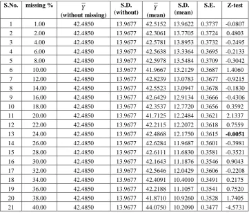
Table 1: Test of significance between

Y

(without missing) and

Y

(after imputation by mean method)

S.No. missing %

_Y

(without missing)

S.D.

(without) _(mean)

Y

S.D. (mean)

S.E. Z-test

1 1.00 42.4850 13.9677 42.5152 13.9622 0.3737 -0.0807

2 2.00 42.4850 13.9677 42.3061 13.7705 0.3724 0.4803

3 4.00 42.4850 13.9677 42.5781 13.8953 0.3732 -0.2495

4 6.00 42.4850 13.9677 42.5638 13.3364 0.3695 -0.2133

5 8.00 42.4850 13.9677 42.5978 13.5484 0.3709 -0.3042

6 10.00 42.4850 13.9677 41.9667 13.2129 0.3687 1.4060

7 12.00 42.4850 13.9677 42.8239 13.0783 0.3677 -0.9215

8 14.00 42.4850 13.9677 42.5523 13.0947 0.3678 -0.1830

9 16.00 42.4850 13.9677 42.6429 12.9134 0.3666 -0.4306

10 18.00 42.4850 13.9677 42.3537 12.7720 0.3656 0.3592

11 20.00 42.4850 13.9677 41.7125 12.2484 0.3621 2.1337

12 22.00 42.4850 13.9677 42.2115 12.2072 0.3618 0.7559

13 24.00 42.4850 13.9677 42.4868 12.1750 0.3615 -0.0051

14 26.00 42.4850 13.9677 42.6284 11.9687 0.3601 -0.3981

15 28.00 42.4850 13.9677 42.6111 11.6830 0.3581 -0.3521

16 30.00 42.4850 13.9677 42.1643 11.1876 0.3546 0.9043

17 32.00 42.4850 13.9677 42.5646 12.0429 0.3606 -0.2208

18 34.00 42.4850 13.9677 42.4091 10.4010 0.3491 0.2175

19 36.00 42.4850 13.9677 42.2188 11.1057 0.3541 0.7520

20 38.00 42.4850 13.9677 41.8710 10.9260 0.3528 1.7405

(6)

[image:6.595.90.508.100.407.2]

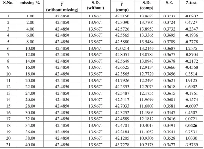
Table 2 : Test of significance between

Y

(after imputation by ratio method)

_Y

S.D.

(without) _(ratio)

Y

S.D. (ratio)

S.E. Z-test

1 1.00 42.4850 13.9677 42.5149 13.9622 0.3737 -0.0801

2 2.00 42.4850 13.9677 42.3099 13.7705 0.3724 0.4703

3 4.00 42.4850 13.9677 42.5709 13.8954 0.3732 -0.2302

4 6.00 42.4850 13.9677 42.5542 13.3365 0.3695 -0.1873

5 8.00 42.4850 13.9677 42.5850 13.5485 0.3709 -0.2695

6 10.00 42.4850 13.9677 42.0367 13.2146 0.3687 1.2160

7 12.00 42.4850 13.9677 42.7998 13.0785 0.3677 -0.8559

8 14.00 42.4850 13.9677 42.5684 13.0947 0.3678 -0.2268

9 16.00 42.4850 13.9677 42.6550 12.9135 0.3666 -0.4637

10 18.00 42.4850 13.9677 42.3573 12.7720 0.3656 0.3492

11 20.00 42.4850 13.9677 41.8163 12.2502 0.3621 1.8470

12 22.00 42.4850 13.9677 42.2417 12.2073 0.3618 0.6726

13 24.00 42.4850 13.9677 42.5645 12.1758 0.3615 -0.2200

14 26.00 42.4850 13.9677 42.5171 11.9701 0.3601 -0.0893

15 28.00 42.4850 13.9677 42.7066 11.6841 0.3581 -0.6187

16 30.00 42.4850 13.9677 42.3731 11.1921 0.3547 0.3154

17 32.00 42.4850 13.9677 42.2630 12.0476 0.3607 0.6156

18 34.00 42.4850 13.9677 42.4861 10.4015 0.3491 -0.0031

19 36.00 42.4850 13.9677 42.2182 11.1057 0.3541 0.7534

20 38.00 42.4850 13.9677 42.1737 10.9328 0.3528 0.8824

21 40.00 42.4850 13.9677 43.5799 10.2270 0.3478 -3.1479

Y

(after imputation by Compromise method)

_Y

S.D.

(without) _(comp)

Y

S.D. (comp)

S.E. Z-test

1 1.00 42.4850 13.9677 42.5150 13.9622 0.3737 -0.0802

2 2.00 42.4850 13.9677 42.3090 13.7705 0.3724 0.4727

3 4.00 42.4850 13.9677 42.5726 13.8953 0.3732 -0.2347

4 6.00 42.4850 13.9677 42.5565 13.3365 0.3695 -0.1936

5 8.00 42.4850 13.9677 42.5880 13.5484 0.3709 -0.2778

6 10.00 42.4850 13.9677 42.0214 13.2140 0.3687 1.2575

7 12.00 42.4850 13.9677 42.8051 13.0784 0.3677 -0.8704

8 14.00 42.4850 13.9677 42.5649 13.0947 0.3678 -0.2172

9 16.00 42.4850 13.9677 42.6525 12.9134 0.3666 -0.4568

10 18.00 42.4850 13.9677 42.3565 12.7720 0.3656 0.3514

11 20.00 42.4850 13.9677 41.7926 12.2495 0.3621 1.9125

12 22.00 42.4850 13.9677 42.2353 12.2073 0.3618 0.6902

13 24.00 42.4850 13.9677 42.5487 12.1755 0.3615 -0.1761

14 26.00 42.4850 13.9677 42.5417 11.9696 0.3601 -0.1574

15 28.00 42.4850 13.9677 42.7033 11.6807 0.3581 -0.6097

16 30.00 42.4850 13.9677 42.3252 11.1903 0.3547 0.4507

17 32.00 42.4850 13.9677 42.4589 12.1812 0.3616 0.0721

18 34.00 42.4850 13.9677 42.4701 10.4013 0.3491 0.0426

19 36.00 42.4850 13.9677 42.2184 11.1057 0.3541 0.7531

20 38.00 42.4850 13.9677 42.1205 10.9306 0.3528 1.0330

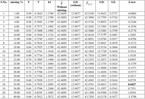
[image:6.595.89.510.435.742.2]

(7)

[image:7.595.69.537.105.424.2]

Y

(after imputation by Ahmed method( using estimator t2)

S.No. missing % V

_Y

without missing

S.D. (without)

t2 (ahmed)

S.D. (ahmed)

S.E. Z-test

1 1.00 0.7643 42.4850 13.9677 42.5150 13.9622 0.3737 -0.0802

2 2.00 0.7722 42.4850 13.9677 42.3090 13.7705 0.3724 0.4726

3 4.00 0.7683 42.4850 13.9677 42.5726 13.8953 0.3732 -0.2346

4 6.00 0.7573 42.4850 13.9677 42.5565 13.3365 0.3695 -0.1936

5 8.00 0.7608 42.4850 13.9677 42.5880 13.5484 0.3709 -0.2778

6 10.00 0.7820 42.4850 13.9677 42.0213 13.2140 0.3687 1.2577

7 12.00 0.7785 42.4850 13.9677 42.8051 13.0784 0.3677 -0.8704

8 14.00 0.7818 42.4850 13.9677 42.5649 13.0947 0.3678 -0.2172

9 16.00 0.7925 42.4850 13.9677 42.6525 12.9134 0.3666 -0.4568

10 18.00 0.7791 42.4850 13.9677 42.3565 12.7720 0.3656 0.3514

11 20.00 0.7716 42.4850 13.9677 41.7925 12.2495 0.3621 1.9128

12 22.00 0.7885 42.4850 13.9677 42.2353 12.2073 0.3618 0.6903

13 24.00 0.7957 42.4850 13.9677 42.5486 12.1755 0.3615 -0.1759

14 26.00 0.7794 42.4850 13.9677 42.5416 11.9696 0.3601 -0.1571

15 28.00 0.7706 42.4850 13.9677 42.6846 11.6836 0.3581 -0.5573

16 30.00 0.7704 42.4850 13.9677 42.3249 11.1903 0.3547 0.4515

17 32.00 0.7820 42.4850 13.9677 42.4584 12.1812 0.3616 0.0737

18 34.00 0.7929 42.4850 13.9677 42.4701 10.4013 0.3491 0.0427

19 36.00 0.7596 42.4850 13.9677 42.2184 11.1057 0.3541 0.7531

20 38.00 0.8245 42.4850 13.9677 42.1201 10.9306 0.3528 1.0342

21 40.00 0.7012 42.4850 13.9677 43.7264 10.2179 0.3477 -3.5697

Y

(after imputation by factor type estimator

T

FT2_{at k1)}

S.No. missing % F V k1

Y

Without missing

S.D.

(without)

T

FT2

S.D. S.E. Z-test

1 1.00 0.99 0.7643 1.1789 42.4850 13.9677 42.5150 13.9622 0.3737 -0.0802 2 2.00 0.98 0.7722 1.1789 42.4850 13.9677 42.3090 13.7705 0.3724 0.4726 3 4.00 0.96 0.7683 1.1799 42.4850 13.9677 42.5726 13.8953 0.3732 -0.2346 4 6.00 0.94 0.7573 1.1902 42.4850 13.9677 42.5565 13.3365 0.3695 -0.1936 5 8.00 0.92 0.7608 1.1905 42.4850 13.9677 42.5880 13.5484 0.3709 -0.2778 6 10.00 0.90 0.7820 1.1734 42.4850 13.9677 42.0218 13.2140 0.3687 1.2565 7 12.00 0.88 0.7785 1.1835 42.4850 13.9677 42.8051 13.0784 0.3677 -0.8704 8 14.00 0.86 0.7818 1.1839 42.4850 13.9677 42.5649 13.0947 0.3678 -0.2172 9 16.00 0.84 0.7925 1.1790 42.4850 13.9677 42.6525 12.9134 0.3666 -0.4568 10 18.00 0.82 0.7791 1.1918 42.4850 13.9677 42.3565 12.7720 0.3656 0.3514 11 20.00 0.80 0.7716 1.2006 42.4850 13.9677 41.7924 12.2495 0.3621 1.9128 12 22.00 0.78 0.7885 1.1908 42.4850 13.9677 42.2353 12.2073 0.3618 0.6903 13 24.00 0.76 0.7957 1.1884 42.4850 13.9677 42.5486 12.1755 0.3615 -0.1759 14 26.00 0.74 0.7794 1.2047 42.4850 13.9677 42.5416 11.9696 0.3601 -0.1571 15 28.00 0.72 0.7706 1.2153 42.4850 13.9677 42.6846 11.6836 0.3581 -0.5573 16 30.00 0.70 0.7704 1.2193 42.4850 13.9677 42.3248 11.1903 0.3547 0.4517 17 32.00 0.68 0.7820 1.2137 42.4850 13.9677 42.4583 12.1812 0.3616 0.0739 18 34.00 0.66 0.7929 1.2085 42.4850 13.9677 42.4701 10.4013 0.3491 0.0427

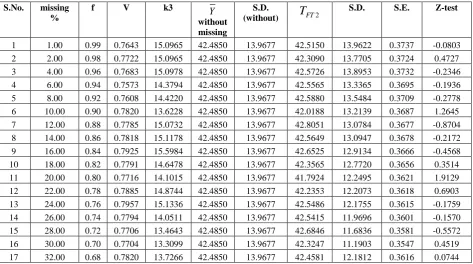
[image:7.595.68.532.453.771.2]

(8)

[image:8.595.46.553.134.449.2]

Y

T

FT2_at

k2)

S.No. missing % F V k2

_Y

S.D.

(without)

T

FT2

S.D. S.E. Z-test

1 1.00 0.99 0.7643 3.3782 42.4850 13.9677 42.5157 13.9622 0.3737 -0.0821

2 2.00 0.98 0.7722 3.3782 42.4850 13.9677 42.3089 13.7705 0.3724 0.4729

3 4.00 0.96 0.7683 3.3644 42.4850 13.9677 42.5726 13.8953 0.3732 -0.2346

4 6.00 0.94 0.7573 3.3578 42.4850 13.9677 42.5565 13.3365 0.3695 -0.1935

5 8.00 0.92 0.7608 3.3474 42.4850 13.9677 42.5880 13.5484 0.3709 -0.2776

6 10.00 0.90 0.7820 3.4727 42.4850 13.9677 41.9930 13.2132 0.3687 1.3345

7 12.00 0.88 0.7785 3.3239 42.4850 13.9677 42.8050 13.0784 0.3677 -0.8702

8 14.00 0.86 0.7818 3.3123 42.4850 13.9677 42.5649 13.0947 0.3678 -0.2172

9 16.00 0.84 0.7925 3.2987 42.4850 13.9677 42.6525 12.9134 0.3666 -0.4569

10 18.00 0.82 0.7791 3.2921 42.4850 13.9677 42.3565 12.7720 0.3656 0.3514

11 20.00 0.80 0.7716 3.2827 42.4850 13.9677 41.7916 12.2495 0.3621 1.9153

12 22.00 0.78 0.7885 3.2668 42.4850 13.9677 42.2352 12.2073 0.3618 0.6904

13 24.00 0.76 0.7957 3.2536 42.4850 13.9677 42.5481 12.1755 0.3615 -0.1744

14 26.00 0.74 0.7794 3.2456 42.4850 13.9677 42.5407 11.9696 0.3601 -0.1546

15 28.00 0.72 0.7706 3.2356 42.4850 13.9677 42.6839 11.6836 0.3581 -0.5554

16 30.00 0.70 0.7704 3.2224 42.4850 13.9677 42.3221 11.1902 0.3547 0.4592

17 32.00 0.68 0.7820 3.2058 42.4850 13.9677 42.4530 12.1814 0.3616 0.0886

18 34.00 0.66 0.7929 3.1888 42.4850 13.9677 42.4698 10.4013 0.3491 0.0436

19 36.00 0.64 0.7596 3.1840 42.4850 13.9677 42.2184 11.1057 0.3541 0.7531

20 38.00 0.62 0.8245 3.1507 42.4850 13.9677 42.1153 10.9304 0.3528 1.0478

21 40.00 0.60 0.7012 3.1722 42.4850 13.9677 43.7165 10.2184 0.3478 -3.5414

Y

T

FT2_at

k3)

S.No. missing %

f V k3

_Y

S.D.

(without)

T

FT2

S.D. S.E. Z-test

1 1.00 0.99 0.7643 15.0965 42.4850 13.9677 42.5150 13.9622 0.3737 -0.0803

2 2.00 0.98 0.7722 15.0965 42.4850 13.9677 42.3090 13.7705 0.3724 0.4727

[image:8.595.63.537.495.759.2]

(9)

18 34.00 0.66 0.7929 14.1445 42.4850 13.9677 42.4701 10.4013 0.3491 0.0427

19 36.00 0.64 0.7596 12.4188 42.4850 13.9677 42.2184 11.1057 0.3541 0.7531 20 38.00 0.62 0.8245 15.8030 42.4850 13.9677 42.1199 10.9306 0.3528 1.0347 21 40.00 0.60 0.7012 10.2930 42.4850 13.9677 43.7256 10.2180 0.3477 -3.5675

5. CONCLUSION

This work analyses the behavior of five imputation methods that can be used for missing data treatment. These methods are analyzed on different percentages of missing data into a common attribute of large data sets. The Ratio method of imputation and Factor type compromised method of imputation provides very good results, even for training sets having a large amount of missing data. In case of mean method of imputation, only at 24% level of missing data, critical value of z score i.e. 0.0051 is less than 5 % level of significance which shows that the results are almost same in case of mean of attribute domain (without missing) and mean attribute domain(with missing) at this percent. In case of ratio method of imputation and , only at 34% level of missing data, critical value of z score i.e. 0.0031 is less than 5 % level of significance which shows that the results are almost same in case of mean of attribute domain (without missing) and mean attribute domain(with missing) at this percent. In case of Ahmed method of imputation, only at 34% level of missing data, critical value of z score i.e. 0.0427 is less than 5 % level of significance which shows that the results are almost same in case of mean of attribute domain (without missing) and mean attribute domain(with missing) at this percent. In case of Factor type compromised method of imputation, at 34% level of missing data, critical value of z score’s are 0.0427, 0.04276 & 0.0427 respectively that is less than 5 % level of significance which shows that the results are almost same in case of mean of attribute domain (without missing) and mean attribute domain(with missing) at this percent.

Although, all the methods are showing approximately correct results at different percentages of missing data but when we compare results of all the methods on same data set, outcome given by ratio method of imputation and Factor type compromised method are more accurate among all. Hence, it may be recommended for imputing the missing values to preprocess the database prior to analysis, so that the quality of the results extracted can be improved.

In future works, the missing data treatment methods will be analyzed in other data sets. Furthermore, in this work missing values were inserted completely at random (MCAR). In a future work, one canl analyze the behavior of these methods when missing values are not randomly distributed. In this case, there is a possibility of creating invalid knowledge. For an effective analysis, it is recommended to inspect not only the error rate, but also the quality of the knowledge induced by the learning system.

6. REFERENCES

[1] Ahmed, M. S., Al-Titi, O., Al-Rawi, Z. and Abu-Dayyeh, W. 2006. Estimation of a population mean using different imputation methods, Statistics in Transition, 7, 6, 1247-1264.

[2] Cochran, W. G. 2005. Sampling Techniques, John Wiley and Sons, New York.

[3] G. E. A. P. A. Batista and M. C. Monard. K-Nearest Neighbour as Imputation Method 2002. Experimental Results. Technical report, ICMC-USP, ISSN-0103-2569. [4] Heitjan, D. F. and Basu, S. 1996. Distinguishing

‘Missing at random’ and ‘missing completely at random’, The American Statistician, 50, 207-213. [5] J. W. Grzymala-Busse and M. Hu. A Comparison of

Several Approaches to Missing Attribute Values in Data Mining 2000. In RSCTC’2000, pages 340–347.

[6] K. Lakshminarayan, S. A. Harp, and T. Samad. 1999. Imputation of Missing Data in Industrial Databases. Applied Intelligence, 11:259–275.

[7] R. J. Little and D. B. Rubin. 1987. Statistical Analysis with Missing Data. John Wiley and Sons, New York, 1987.

[8] Rao, J. N. K. and Sitter, R. R. 1995. Variance estimation under two-phase sampling with application to imputation for missing data, Biometrica, 82, 453-460.

[9] Reddy, V. N. 1978. A study on the use of prior knowledge on certain population parameters in estimation, Sankhya, C, 40, 29-37.

[10]Rubin, D. B. 1976. Inference and missing data, Biometrica, 63, 581-593.

[11]Shukla, D. 2002. F-T estimator under two-phase sampling, Metron, 59, 1-2, 253-263.

[12]Shukla, D. and Thakur, N. S. 2008. Estimation of mean with imputation of missing data using factor-type estimator, Statistics in Transition, 9, 1, 33-48.

[13]Thakur, N. S., Yadav Kalpana, and Pathak S. 2012. Some imputation methods in double sampling scheme for estimation of population mean, IJMER, Vol.2, Issue.1 Jan-Feb 2012 pp-200-207.

[14]Thakur, N. S., Yadav Kalpana, and Pathak S. 2011.Estimation of mean in presence of missingdata under two-phase sampling scheme, JRSS,Vol 4, issue 2,93-104.

[15]Singh, S. 2009. A new method of imputation in survey sampling, Statistics, Vol. 43, 5 , 499 - 511.

[16]Singh, S. and Horn, S. 2000. Compromised imputation in survey sampling, Metrika, 51, 266-276.

[17]Singh, V. K. and Shukla, D. 1993. An efficient one parameter family of factor - type estimator in sample survey, Metron, 51, 1-2, 139-159.