BIROn - Birkbeck Institutional Research Online
Gutin,
G.Z. and Reidl,
Felix and Wahlström,
M. and Zehavi,
M.
(2018) Designing deterministic polynomial-space algorithms by color-coding
multivariate polynomials. Journal of Computer and System Sciences 95 , pp.
69-85. ISSN 0022-0000.
Downloaded from:
Usage Guidelines:
Please refer to usage guidelines at
or alternatively
arXiv:1706.03698v2 [cs.DS] 19 Dec 2017
Designing Deterministic Polynomial-Space
Algorithms by Color-Coding Multivariate
Polynomials
∗
Gregory Gutin
1, Felix Reidl
1, Magnus Wahlstr¨
om
1, and Meirav
Zehavi
21
Royal Holloway, University of London, TW20 0EX, UK
2
University of Bergen, Norway
Abstract
In recent years, several powerful techniques have been developed to design randomized polynomial-space parameterized algorithms. In this paper, we introduce an enhancement of color coding to design determin-istic polynomial-space parameterized algorithms. Our approach aims at reducing the number of random choices by exploiting the special structure of a solution. Using our approach, we derive polynomial-spaceO∗(3.86k
)-time (exponential-space O∗(3.41k
)-time) deterministic algorithm for k -Internal Out-Branching, improving upon the previously fastest expo-nential-space O∗(5.14k
)-time algorithm for this problem. (The notation
O∗hides factors polynomial in the input size.) We also design
polynomial-space O∗((2e)k+o(k)
)-time (exponential-spaceO∗(4.32k
)-time) determin-istic algorithm fork-Colorful Out-Branchingon arc-colored digraphs andk-Colorful Perfect Matchingon planar edge-colored graphs. In
k-Colorful Out-Branching, given an arc-colored digraph D, decide whether D has an out-branching with arcs of at least k colors. In k -Colorful Perfect Matching, given an undirected graph G, decide whether G has a perfect matching with edges of at least k colors. To obtain our polynomial space algorithms, we show that (n, k, αk)-splitters (α>1) and in particular (n, k)-perfect hash families can be enumerated one by one with polynomial delay using polynomial space.
1
Introduction
In this paper, we modify color coding to treat multivariate polynomials, and thus
design an improved deterministic polynomial-space algorithm fork-Internal
∗Gutin was partially supported by Royal Society Wolfson Research Merit Award, Reidl and
Out-Branching (k-IOB). Before we elaborate on this problem and our con-tribution, let us first review related previous works that motivate our study. In recent years, several powerful algebraic techniques have been developed to design
randomizedpolynomial-space parameterized algorithms. The first approach was introduced by Koutis [1], strengthened by Williams [2], and is nowadays known as the multilinearity detection technique [3]. Roughly speaking, an application of this technique consists of reducing the problem at hand to one where the objective is to decide whether a given polynomial has a multilinear monomial, and then employing an algorithm for the latter problem as a black box.
One of the huge breakthroughs brought about by this line of research was
Bj¨orklund’s [4] proof that Hamiltonian Path is solvable in time O∗(1.66n)
by a randomized algorithm, improving upon the 50 year old O∗(2n)-time1
al-gorithm [5]. The existence of a deterministic O∗((2
−ε)n)-time algorithm for
Hamiltonian Path, for a fixedε >0, is still a major open problem. Further,
Bj¨orklund’s result is on undirected graphs, and the existence of anO∗((2
−ε)n
)-time algorithm forHamiltonian Pathon digraphs, for a fixedε >0, is another
interesting open problem.
Shortly afterwards, Bj¨orklund et al. [6] have transformed the ideas in [4]
into a powerful technique to design randomized polynomial-space algorithms,
referred to as narrow sieves. This technique is also based on the analysis of
polynomials, but it is applied quite differently. Here one associates a monomial with each “potential solution” in such a way that actual solutions correspond to unique monomials while incorrect solutions appear in pairs. Thus, the poly-nomial summing these mopoly-nomials, when evaluated over a field of characteristic 2, is not identically 0 if and only if the input instance of the problem at hand is a yes-instance. In this context, the relevance of the Matrix Tree Theorem was
already noted by Gabizonet al. [7].
The narrow sieves technique, proven to be of wide applicability on its own, later branched into several new methods. The one most relevant to our study
was developed by Bj¨orklund et al. [8] and was translated into the language of
determinants by Wahlstr¨om [9]. Here, the studied problem wasS-Cycle(or
S-Path), where the goal is to determine whether an input graph contains a cycle
that passes through all the vertices of an input setS of sizek. Wahlstr¨om [9]
considered a determinant-based polynomial (computed over a field of character-istic 2), and analyzed whether there exists a monomial where the variable-set
representingS is present. Very recently, Bj¨orklund et al. [10] utilized the
Ma-trix Tree Theorem to improve an FPT algorithm fork-IOB, where we are asked
to decide whether a given digraph has ak-internal out-branching. Recall that
anout-treeT is an orientation of a tree with only one vertex of in-degree zero
(called theroot). A vertex ofT is aleafif its out-degree inT is zero; non-leaves
are calledinternal vertices. Anout-branchingof a digraphD is a spanning
sub-graph ofD, which is an out-tree, and an out-branching isk-internal if it hasat
leastkinternal vertices.
Bj¨orklundet al. [10] cleverly transformedk-IOB into a new problem, where
the goal is to decide whether a given polynomial (computed over a field of
characteristic 2 to avoid subtractions) has a monomial with at leastk distinct
variables.
In this paper, we present an easy-to-use2 modification of color coding for
designing deterministic polynomial-space parameterized algorithms, inspired by the principles underlying the above mentioned techniques. (A slight modifica-tion of our approach can be used to design faster, exponential-space algorithms, but we believe that the main value of the approach is for polynomial-space algorithms.) We will show that our approach brings significant speed-ups to
al-gorithms fork-IOB. Roughly speaking, our approach can be applied as follows.
• Identify a polynomial such that it has a monomial with at leastkdistinct
variables (called awitnessing monomial) if and only if the input instance
of the problem at hand is a yes-instance. It should be possible to efficiently evaluate the polynomial (black box-access is sufficient here).
• Color the variables of the polynomial with k colors using a
polynomial-delay perfect hash-family. To improve the running time of this step, we
apply a problem-specificcoloring guide to reduce the number of ‘random’
colors. Given ak-coloring, we obtain a smaller polynomial by identifying
all variables of the same color.
• Use inclusion-exclusion to extract the coefficient of a colorful monomial
from the reduced polynomial. By the usual color-coding arguments, if the coefficient is not equal to zero then the original polynomial contained a witnessing monomial.
While we were unable to obtain non-trivial coloring guides to the following prob-lems, even limited application of our approach is useful for designing polynomial-space algorithms for these problems. It would be interesting to obtain non-trivial coloring guides for the problems.
Colorful Out-Branchings and Matchings Every subgraph-search problem can be extended quite naturally by imposing additional constraints on the solu-tion, for example by letting the input graph have labels or weights. One class of such constraints states that a required subgraph of an edge-colored graph has
to bek-colorful, i.e. to contain edges of at leastkcolors.
One prominent problem is Rainbow Matching3(also known as
Multi-ple Choice Matching), defined in the classical book by Garey and Johnson
[11]. Itai et al. [12] showed, already in 1978, that Rainbow Matching is
NP-complete on bipartite graphs. Three decades later, Le and Pfender [13]
re-visited this problem and showed that it isNP-hard on several restricted graph
classes, which include (among others) paths, complete graph and P4-free
bi-partite graphs in which every color is used at most twice. Further examples of
2In particular, no dynamic programming/recursive algorithms are required.
3In the problem, given an edge-colored graphG and an integer k, the aim is to decide
subgraph problems with color constraints can be found in a survey by Mikio and Xueliang [14]. In this paper, we focus on two color-constrained problems: given
an edge-colored graph and an integerk, we ask for either ak-colorful spanning
tree/outbranching or ak-colorful perfect matching.
We first rely on the Matrix Tree Theorem to present a deterministic
poly-nomial-spaceO∗((2e)k+o(k))-time (exponential-spaceO∗(4.32k)-time) algorithm
fork-Colorful Out-Branching, defined as follows:
Input: A arc-colored digraphD and an integerk
Problem: DoesD have ak-colorful out-branching?
Colorful Out-Branchingparametrised by k
We argue in Section 5 thatk-Colorful Out-BranchingisNP-hard on
vari-ous restricted graph classes such as cubic graphs.
Next, we rely on a Pfaffian computation to present a deterministic
polynomial-spaceO∗((2e)k+o(k))-time (exponential-space
O∗(4.32k)-time) algorithm for
k-Colorful Perfect Matchingon planar graphs, defined as follows:
Input: A planar edge-colored graphGand an integerk
Problem: DoesGhave ak-colorful perfect matching?
Planar Colorful Perfect Matchingparametrised by k
We will show in Section 6 by a simple reduction that Planar k-Colorful
Perfect Matching is NP-hard even on planar graphs of pathwidth 2. It is
worthwhile to note that whileRainbow Matchingcan be viewed as a special
case of the well-known 3-Setk-Packingproblem, and in particular, a solution
for Rainbow Matching is small (containing only 2k vertices and k colors),
the case ofk-Colorful Perfect Matching is different in the sense that a
solution is necessarily large since not everyk-colorful matching can be extended
to a perfect matching.
k-Internal Out-Branching By utilizing the method of bounded search trees on top of the above machinery, in Section 4, we present a deterministic
polynomial-spaceO∗(3.86k)-time (exponential-space
O∗(3.41k)-time) algorithm for the
prob-lemk-Internal Out-Branching (k-IOB), defined as follows:
Input: A digraphDand an integer k
Problem: DoesD have ak-internal out-branching?
Internal Out-Branching (IOB)parametrised by k
The undirected version ofk-IOB, calledk-Internal Spanning Tree (k-IST),
Input: A graphGand an integerk
Problem: DoesGhave ak-internal spanning tree?
Internal Spanning Tree (IST)parametrised by k
Note that k-IOB is a generalization of k-IST since the latter can easily be
reduced to k-IOB on symmetric digraphs, i.e. digraphs in which every arc is
on a directed cycle of length 2. Since k-IST is NP-hard (Hamiltonian Path
appears as a special case fork=n−2) it follows that so isk-IOB. The latter
is, however, polynomial time solvable on acyclic digraphs [15]. While acyclic
digraphs are precisely digraphs of directed treewidth 0, it turns out thatk-IOB
isNP-hard already for digraphs of directed treewidth 1 [16]. By constrast, the
Directed Hamilton Pathproblems is polynomial-time solvable on digraphs
of directed treewidtht[17] iftis a constant. Thek-IOB problem a priori seems
more difficult than the well-known k-Path problem (decide whether a given
digraph has a path on k vertices) since a witness of a yes-instance of k-path
is a subgraph of size k, that is, a path on k vertices. However, it is easy to
see that a witness of a yes-instance ofk-IOB (which has an out-branching) can
be a subgraph of size 2k−1, that is, an out-tree withk internal vertices and
k−1 leaves. This simple but crucial observation lies at the heart of previous
algorithms fork-IOB.
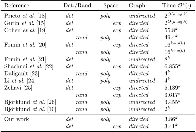
Reference Det./Rand. Space Graph TimeO∗(·)
Prietoet al. [18] det poly undirected 2O(klogk)
Gutinet al. [15] det exp directed 2O(klogk)
Cohenet al. [19] det exp directed 55.8k
rand poly directed 49.4k
Fominet al. [20] det exp directed 16k+o(k)
rand poly directed 16k+o(k)
Fominet al. [21] det poly undirected 8k
Shachnaiet al. [22] det exp directed 6.855k
Daligault [23] rand poly directed 4k
Li et al. [24] det poly undirected 4k
Zehavi [25] det exp directed 5.139k
rand exp directed 3.617k
Bj¨orklundet al. [26] rand poly undirected 3.455k
Bj¨orklundet al. [10] rand poly undirected 2k
Our work det poly directed 3.86k
[image:6.612.141.471.391.614.2]det exp directed 3.41k
Table 1: Previously known FPT algorithms fork-IOBandk-IST.
Parameterized algorithms fork-IST andk-IOB were first studied by Prieto and
fixed-parameter tractable (FPT), i.e. admit deterministic algorithms of running time
O∗(f(k)), where f(k) is an arbitrary recursive function depending on the
pa-rameter k only. Moreover, both papers showed that f(k) = 2O(klogk). Since
then several papers improved complexities of deterministic and randomized al-gorithms for both problems; we list these alal-gorithms in Table 1. We also remark that approximation algorithms, exact exponential-time algorithms and
kernel-ization algorithms for bothk-IOB andk-IST were extensively studied, but the
survey of such results is beyond the scope of this paper.
Our polynomial-space algorithm fork-IOBis faster, in terms off(k), than
not only the previously fastestexponential-spaceO∗(5.139k)-time deterministic
algorithm fork-IOB by Zehavi [25], but also the previously fastest
polynomial-spaceO∗(4k)-time deterministic algorithm fork-IST of Liet al. [24]. In contrast,
it is not known how to design a deterministic polynomial-spaceO∗((4
−ε)k)-time
algorithm for the k-Path problem. Indeed, a deterministic polynomial-space
O∗(4k+o(k))-time algorithm fork-Pathhas been known since 2006 [27],4yet so
far no improvements without the help of exponential space [28, 25] have been made.
The rest of the paper is organized as follows. In the next section, we in-troduce necessary preliminary material. Section 3 describes our approach in detail. The main contents of the next three sections were discussed above. In Section 7, we prove a derandomization theorem forming part of our approach. In Section 8, we show a proposition, which assists us in upper-bounding run-ning times of exponential-space algorithms. We conclude the paper in Section 9 discussing some open problems.
2
Preliminaries
We assume the reader is familiar with basic concepts and notations in Graph Theory and Linear Algebra, and refer readers to textbooks in Graph Theory [29, 30] and Linear Algebra [31] if additional details are required.
We will make use of the tighter version of Stirling’s approximation due to Robbins [32], which states that
√
2πk k
e
k
e1/(12k+1)6k!6√2πk k e
k
e1/12k.
Forα>1 we will frequently use the function
τ(α) =1−α1α−1e,
with the convention thatτ(1) =e. We will sometimes use the symbol• in the
following to denote a variable whose value is arbitrary.
4Although Chen et al. [27] do not explicitly prove that the space complexity of their
Operations on polynomials For a polynomial P and a monomial M, we
let coefP(M) denote the coefficient ofM in P.For a polynomialP(x1, . . . , xn)
and subset of the variables C ⊆ {x1, . . . , xn}, letP/C denote the polynomial
obtained from P by replacing all variables in C by a new variable yC. We
extend this notation to partitions C := C1⊎. . .⊎Cp and letP/C denote the
polynomial (. . .((P/C1)/C2). . .)/Cp.
Structural Observation It is not hard to decide whether a digraphD has
an out-branching in linear time: D contains an out-branching if and only ifD
has only one strongly connected component without incoming arcs (see, e.g., [29]). Thus, in what follows, whenever we discuss problems where a solution
is in particular an out-branching, we will assume that the digraph D under
consideration contains an out-branching.
Matrix Tree Theorem In 1948 Tutte [33] proved the (Directed) Matrix Tree Theorem, which shows that the number of out-branchings rooted at the same
vertexrin a digraphDcan be found efficiently by calculating the determinant
of a certain matrix derived fromD. Here, we require a generalization of this
theorem, whose derivation from the original theorem is folklore (a proof can be found, e.g., in [10]).
The(symbolic) Kirchoff matrix K=K(D) of a directed multigraphD onn
vertices is defined as follows, where we assume that the vertices are numbered
from 1 ton:
Kij =
X
ℓi∈A(D)
xℓi ifi=j, −xij ifij∈A(D),
0 otherwise,
(1)
whereA(D) is the arc set ofD.
In what follows, [n] :={1,2, . . . , n}. Fori∈[n] we denote byK¯i(D) the
ma-trix obtained fromK(D) by deleting theith row and theith column. Moreover,
letBidenote the set of out-branchings rooted ati. The following version of the
(Directed) Matrix Tree Theorem implies a natural one-to-one correspondence
between the monomials of det (K¯i(D)) and the out-branchings inBi.
Theorem 1. For every directed multigraph D with symbolic Kirchoff matrix
K(D)andi∈V(D),det (K¯i(D)) =
X
B∈Bi Y
ij∈A(B)
xij.
Planar Graphs, Perfect Matchings and Pfaffians The Pfaffian is an im-portant tool for polynomial-time counting algorithms, closely related to perfect
matchings of a graph. A square matrix M ∈ Rn×n is skew-symmetric if for
everyi, j∈[n] it holds thatM(i, j) =−M(j, i). LetM be skew-symmetric and
of even dimension 2n. For every partition of [2n] into pairs{{ia, ja} |a∈[n]},
define a corresponding permutation (i1, j1, . . . , in, jn) of [2n] whereia < ja for
every partition into pairs, and let Πndenote the set of permutation of partitions
of [2n]. Then the Pfaffian ofM can be defined as
pf(M) = X
π∈Πn
σ(π)
n Y
t=1
M(π(2t−1), π(2t)),
whereσ(π) =±1 is a sign term referred to as thesignature of the permutation.
The Pfaffian can be efficiently computed; in particular, pf(M) = (det(M))2.
Among other applications, the Pfaffian can be used to count the number of perfect matchings of a planar graph by computing an orientation of the graph where every signature in the above sum is +1; see Section 6.
Hash Families and Splitters The notion of perfect hash family was
em-ployed by Alonet al. [34] when they introduced the framework of color coding.
Splitters are generalizations of perfect hash families; both are defined below.
Let ¯x= (x1, . . . , xn)∈[t]n be a vector andI ={p1, . . . , p|I|} ⊆ [n], where
p1 < · · · < p|I|. Then ¯x[I] := (xp1. . . , xp|I|). We say that ¯x[I] partitions I almost equallyif the cardinalities of the sets{i∈I: xi=q},q∈[t] differ from
each other by at most 1.
Definition 2 (Splitter). An (n, k, t)-splitter is a family of vectors S ⊆ [t]n such that for every index setI∈ [nk]
there exists at least one vectorx¯∈ S such thatx¯[I] partitions I almost equally. The sizeof the splitter is |S|.
Definition 3 (Perfect hash family). An (n, k, k)-splitterS ⊆ [k]n is called
an(n, k)-perfect hash family. In other words, for every index setI∈ [nk]
there exists a vectorx¯∈ S such that ¯x[I]is a permutation of [k].
Note that the members of an (n, k, t)-splitter can equivalently be interpreted as
vectors from [t]n, as functions that map [n] into [t], or as partitions of [n] intot
blocks.
3
Our Approach
Let us now elaborate on the four main steps that constitute our approach.
1 Polynomial Identification
Associate variablesX={x1, x2, . . . , xn}with some elements (e.g., vertices
or edges) of the input instance and identify a polynomial P(x1, . . . , xn)
over the reals that satisfies the following properties.
– P(x1, . . . , xn) has a monomial with at leastkdistinct variables, called
awitnessing monomial W, if and only if the input instance is a yes-instance;
– All witnessing monomials of P(x1, . . . , xn) (in standard form) have
– For any partitionCofXintokblocks and any assignment of the
vari-ablesy1, . . . , yk(yicorresponds to blocki), the polynomial (P/C)(y1, . . . , yk)
can be evaluated efficiently using polynomial space.5
2 Derivation of Coloring Guides
Define a partition S = S1⊎S2. . . Sp⊎S⊥ of the variables X with the
following property: if there exists a witnessing monomial W, then in
particular there exists such a monomial with |W ∩Si| = 1 for i ∈ [p]
and |W ∩S⊥| = k−p. We say that such a partition S is a coloring
guide. Note that we might consider more than one guide, e.g. by a suit-able branching procedure. In this case, we apply the following steps to all the generated guides and the above property needs to hold for at least one of the generated guides.
3 Color Coding & Derandomization
Color the variablesS⊥withk−pcolors uniformly at random and let the
re-sulting color partition beC:=C1⊎C2⊎. . .⊎Ck (whereCi =Sifori6p
and S
i>pCi =S⊥). To derandomize this step, use an (n, k−p)-perfect
hash family F that is enumerable with polynomial space (cf. Theorem 4
stated shortly) to colorS⊥. Proceed with the next step for every
color-ingC.
4 Coefficient Extraction
Test whetherP/Ccontains a monomialW in which all variablesy1, . . . , yk
appear with a standard inclusion-exclusion algorithm. For example, we
can apply Lemma 6 stated shortly forP/Cby evaluating the corresponding
Q(y1, . . . , yk)6= 0 atyi= 1 for alli∈[k]. Clearly, such a W exists if and
only if Q(1,1, . . . ,1) 6= 0. If so, conclude that P contains a witnessing
monomial and return that the instance is a yes-instance.
We remark that Naor et al. [35] proved that an (n, k)-perfect hash family of
sizeO∗(ek+o(k)) can be computed in timeO∗(ek+o(k)). They claimed that their
construction can be modified so that it is not required to compute the family “at once”, but the vectors in the family can be enumerated with polynomial delay. However, a proof of the latter claim has not been published (the proof was deferred to a full version of that paper which never appeared).
In Section 7 we prove a more general theorem from which this claim can be derived as a corollary. Importantly, our construction requires only polynomial
space, a feature that the construction by Naoret al. does not achieve.
Theorem 4. There exists an (n, k, αk)-splitter of sizekO(1)τ(α)k+o(k)lognfor everyα>1. Moreover, the members of the family can be enumerated determin-istically with polynomial delay using polynomial space.
In case we are interested in polynomial space, we compute F simply as an
(n, k−p)-perfect hash family. Otherwise, we computeFas an (n, k−p, α⋆(k
−p
))-splitter with a suitable constant α⋆
≈ 43. In the latter scenario, we can run
Steps 3 and 4 of our approach in time O∗(τ(α⋆)k−p+o(k)2α⋆(k−p)+p
). This
requires exponential space, as there are α⋆(k−pk )+p
monomials for which we
need to check divisibility (see Lemma 6), but for everyI⊆[α⋆(k−p) +p], we
would evaluateP−I only once rather than once per such monomial. Then, we
can rely on the following result proved in Section 8.
Proposition 5. There exists a constant α⋆ ≈ 4
3 such that using an (n, k −
p, α⋆(k−p))-splitter and exponential space, we can run Steps 3 and 4 of our approach in timeO∗(4.312k−p2p).
In the context of randomized algorithms, a slightly weaker result (O∗(4.314k))
was obtained by H¨uffneret al. [36].
The following Lemma 6 provides a way to extract from P only monomials
divided by a certain term, the crucial operation in step 4 . The lemma is
a modification of a lemma by Wahlstr¨ohm [9] for polynomials over a field of characteristic two.
Lemma 6 (Monomial sieving). Let P(x1, . . . , xn) be a polynomial over re-als, and J ⊆[n] a set of indices. For a set I ⊆[n], define P−I(x1, . . . , xn) =
P(y1, . . . , yn),whereyi= 0for i∈I andyi=xi otherwise. Define
Q(x1, . . . , xn) = X
I⊆J
(−1)|I|P
−I(x1, . . . , xn). (2)
Then, for any monomialM divisible byΠi∈Jxi, we havecoefQ(M) = coefP(M), and for every other monomialM we havecoefQ(M) = 0.
Proof. Consider a monomialM with non-zero coefficient inP.Observe first that
for everyI⊆[n], we have coefP−I(M) = coefP(M) if no variablexi withi∈I
occurs inM, and coefP−I(M) = 0, otherwise. Now, if Πi∈Jxi dividesM, then
out of the 2|J| evaluations for I
⊆J, the monomial M occurs in exactly one
(namely,I=∅). Thus, coefQ(M) = coefP(M).
If Πi∈Jxidoes not divideM, note thatJ′={i∈J :xi does not divideM},
is nonempty and observe that coefP−I(M) = coefP(M) for everyI⊆J
′.Thus,
sum (2) forM only is
X
I⊆J
(−1)|I|M = X
I⊆J′
(−1)|I|M =M X
I⊆J′
(−1)|I|=M(1−1)|J′|= 0.
Applying the above results individually to every monomial inP accounts for all
occurrences of monomials in the sum definingQ; the result follows.
4
k
-Internal Out-Branching
In a digraph D, a matching is a collection of arcs without common vertices.
Lemma 7. The following statements hold.
(i) LetT be an out-tree withk>0 internal vertices. ThenT has a matching of size at least k/2.
(ii) LetD= (V, A)be a digraph containing an out-branching, andM a match-ing in D. Then, in polynomial time, we can find an out-branching ofD
for which no arc ofM has both end-vertices as leaves.
Proof. (1) We prove it by induction on k >0. The claim obviously holds for
k= 0, so assume thatk >1. Theheight of a vertex v in T is the length of a
longest path from v to a leaf of T reachable from v. Letki be the number of
vertices ofT of heighti. Observe thatk1>k2 and thatT has a matchingM1
withk1 edges whose vertices are some leaves and all vertices of height 1. Let
T′ be an out-tree obtained fromT by deleting all leaves and vertices of height
1. Observe that T′ has k
−k1−k2 internal vertices and thus by induction
hypothesisT′ has a matchingM
2 of size at least (k−k1−k2)/2 >k/2−k1.
Thus, the matchingM1∪M2 ofT is of size at leastk/2.
(2) Let B be an out-branching ofD and suppose that both end-vertices of
some arc xy of M are leaves inB. Then add xy to B and delete zy from B,
wherezis the in-neighbor ofy inB. In the resulting out-branchingB′,xis an
internal vertex. Notice thatzy does not belong toM. Hence,B′ contains one
more arc ofM thanB. Starting with an arbitrary out-branching and repeating
the above exchange operation at most|M|times, we will get an out-branching
in which no arc of M has both end-vertices as leaves. This process can be
completed in polynomial time.
We now prove the main theorem of this section.
Theorem 8. There exists a deterministic polynomial-space O∗(3.86k)-time al-gorithm fork-Internal Out-Branching.
Proof. LetD be a digraph,V(D) = [n], andM a maximum matching inD of
size t. By Lemma 7, we may assume thatk/2 6 t 6k as otherwise we can
solvek-IOB onD in polynomial time: Fort < k/2, no out-tree withkinternal
vertices exists and fort > k, we can construct a solution in polynomial time.
Now we will follow our approach.
1 : We associate one variable xv with every vertex v ∈ [n]. Replace every
variablexij in (1) byxi and observe that now by Theorem 1 we have that if the
polynomial det(K¯r(D)) over variables x1, . . . , xn contains a monomial with at
leastk different variables, then there exists an out-branching rooted at rwith
at leastk internal vertices. Note that for ak-coloringC of the variables we can
evaluate the polynomial det(K¯r(D))/C over variablesy1, . . . , yk in polynomial
time. We guess the root vertexr and fix it for the following steps.
2 : For everyc∈[k]∪{0}, we consider all setsM′ofcedges ofM in which both
(the edges of M \M′ contain at least one internal vertex in some k-internal
out-branchings by Lemma 7 (ii)).
For the current choice ofM′, our coloring guideSlooks as follows.6 For every
arcuv∈M′, we add the sets{u}and{v}toS. For every arcxy∈M\M′, we
add the set{x, y}. Finally,S⊥:=V(D)\V(M) contains all vertices outside of
the matching.
3 : Witht+cinternal vertices of the out-tree inV(M) there arek−t−cvertices
left to be located inV(D)\V(M). Using an (n, k−t−c)-perfect hash family, we
color the vertices ofS⊥ and obtain ak-coloringC:=C1⊎C2⊎. . .⊎Ct+c⊎C⊥
of the variables X by combining the coloring from the hash family with the
coloring guideS.
4 : We apply Lemma 6 to the polynomial det(Kr¯(D))/C over y1, . . . , yk to
search for a monomial that contains allk variables. If such a monomial exists,
then det(Kr¯(D)) contains a monomial withkdistinct variables and we conclude
thatD contains an out-branching rooted atrwithk or more internal vertices.
Otherwise, if we have not yet exhausted all colorings in the hash family, we
return to Step 3, and if we have not yet exhausted all guesses for M′, we
return to Step 2 . If neither of these conditions is true, we conclude that there
is nok-internal out-branching rooted atr.
Let us analyse the exponential partf(k) of the running time for the above steps.
Step 2 to 4 take time at most
k−t X c=0 t c
τ(1)(k−t−c)(1+o(1))2k =
k−t X c=0 t c
e(k−t−c)(1+o(1))2k,
using the (n, k −t−c)-perfect hash family from Theorem 4 (with α = 1).
Consider the term ct
e−(t+c)and setc =βt, whereβ
∈(0,1). Using the
well-known bound βtt
6 2tH(β), where H(β) =
−log(ββ(1
−β)1−β), we arrive
at
t
βt
e−t(1+β)6(ββ(1−β)1−βe1+β)−t6
e+ 1
e2
t
.
The second inequality above follows from the fact that min0<β<1g(β) = e+1e ,
where g(β) = ββ(1
−β)1−βeβ, which can be verified by differentiating g(β).
It is easy to verify that βtt
e−t(1+β) 6 (e+1
e2 )t for β = 0 and β = 1 as well.
Therefore, k−t X c=0 t c
e(k−t−c)(1+o(1))2k6k
e+ 1
e2
t
(2e)k(1+o(1)).
Observe that ee+12 < 1 and thus (
e+1
e2 )t decreases monotonically as t grows.
Therefore, (ee+12 )t6(ee+12 )k/2 as t>k/2.Thus,f(k) is bounded from above by
k(4(e+ 1))k(1+o(1))/2< k3.857k forklarge enough. Since all of the above steps
require polynomial space, the algorithms requires polynomial space as well.
6Formally, we somewhat abuse terminology and notation for coloring guide here, but since
If (D, k) is a positive instance of k-IOB, then we can find a k-internal
out-branching of D also in polynomial space and time O∗(3.857k) by the usual
self-reducibility argument: Consider every arcaof D at a time and remove it
fromDif (D−a, k) is a positive instance ofk-IOB until no arc can be removed.
The non-empty remaining graph spans an out-branching withkinternal leaves.
Let us now see how our approach yields a faster algorithm if we use expo-nential space.
Theorem 9. There exists an exponential-space O∗(3.41k)-time algorithm for
k-Internal Out-Branching.
The exponential-space strategy will use the exponential-space version of the
color-coding and sieving result, but we will in addition usetruncatedfast subset
convolution to further speed up the algorithm, by rolling up the ct
guesses in
Step 2 and the applications of Lemma 6 into a single exponential-space
com-putation. This was presented in Bj¨orklundet al. [37] (called trimmed Moebius
inversion).
Proof. We will present the proof as close to the structure of the proof of Theo-rem 8 as possible. However, since the truncated fast subset convolution does not strictly speaking follow the coloring guide method, some discrepancies between
the proofs are unavoidadble. LetD be a digraph with vertex setV = [n].
1 : As before, letM a maximum matching inDof sizetwithk/26t6k. Also
guess a root vertexrand keep it fixed through the following steps. Number the
edges ofM as M ={e1, . . . , et}. With every edge ei ∈M we associate three
variablesxi,x′i,xi′′, and with every vertexv∈V\V(M) we associate a variable
xv. Further, for every edge ei=uv∈M define x(u) = xix′i and x(v) =xix′′i,
and for every other vertex v ∈ V \V(M) define x(v) = xv. Replace every
variablexij in (1) byx(i). We will sieve the polynomial det(Kr¯(D)) according
to two modes for every edgeei ∈M: Either only one endpoint ofei is internal
in the out-branching, in which case we sieve for the variablexi, or both are, in
which case we sieve for bothx′
iandx′′i. Using truncated fast subset convolution,
we will sieve for these options in parallel.
2 +3: Guess the number c ∈ [k−t]∪ {0} of edges of M for which both
endpoints are internal in the solution, but do not guess an explicit subsetM′.
Letk′ :=k
−t−cbe the number of internal vertices of the sought solution that
lie outsideV(M), and recall the constantα⋆ from Proposition 5. Further fix a
coloringf of the vertices ofV \V(M) into α⋆
·k′ colors, and assume that the
k′ internal vertices not present inM all receive distinct colors byf. Repeat the
following steps for every choice off from an (n, k′, α⋆k′)-splitter.
4 : We now describe the improved parallel sieving strategy. Define X =
{xi, x′i, x′′i | i ∈ [t]}, and let P(X, Y) be the result of replacing every
vari-ablexj,j ∈V \V(M), in det(Kr¯(D)) byyf(j). Consider one particular choice
M′
⊆ M, |M′
| = c, of edges where both endpoints are assumed to be
inter-nal vertices in the solution. We would then be seeking a monomial ofP(X, Y)
which contains both variablesx′
every edgeei∈(M\M′), and additionally variables ofk′ further colorsyℓ∈Y.
Combining this across all choices ofM′with
|M′
|=c, we will thus want to run
the sieving algorithm for the family of sets
Fc:= n
{x′i}i∈I∪ {x′′i}i∈I∪ {xi}i∈[t]\I I∈
[t]
c
o ×
[α⋆k′]
k′
.
For eachF ∈ Fc, letQF(X, Y) be polynomial defined in Lemma 6. Up to the
choice of c and f, the instance is positive if and only if there is some F such
thatQF(X, Y)6= 0, and we can useX =1, Y =1for the evaluation, where1
denotes a vector with all components equal 1.
Using the truncated fast subset convolution, we can compute all evaluations
QF(1,1) as above in time proportional to the number of subsets of setsF ∈ Fc,
up to a polynomial factor [37]. Concretely, letIc ={I ⊆F |F ∈ Fc}. Then
the truncated fast subset convolution runs in timeO∗(
|Ic|), and we repeat this
procedure for every choicecand for every memberf of the (n, p, α⋆k′)-splitter,
Running time. To simplify the analysis of the running time, we write Jc =
{I∩X |I ∈ Ic}. Then |Ic| 6|Jc| ·2α
⋆k′
, and the product of the size of the
splitter and 2α⋆k′
can be bounded asO∗(4.312k′) as in Proposition 5. It remains
to bound|Jc|. We further splitJcintoc+1levels, where a setI∈ Jcbelongs to
leveli, 06i6c, if there are exactlyiedgesej∈M such thatI∩ {x′j, x′′j} 6=∅.
Thus, the number of sets at leveliof Jc equals
t i 3i t−c X j=0
t−i j 6 t i
3i2t−i,
where the factor of 3 comes from the three options{x′
j},{x′′
j},{x′j, x′′j}and the
expression in the summation corresponds to whetherxj ∈I for the remaining
edges. Note that the upper bound is essentially tight assumingt−c >(t−i)/2.
Therefore, if we split out the total work per level, we get
max
i∈[c]∪{0} t
i
3i2t−i4.312k−t−c= 2t4.312k−t−c max
i∈[c]∪{0} t
i
1.5i. (3)
To obtain an upper bound for (3), we will use the following observation.
Claim. Let b be a real, t an integer, and xan integral variable. The function
g(x) = xt
bx monotonically increases if and only if x6 b(t+1)
b+1 .
Proof. It suffices to observe thatg(x)/g(x−1)>1 if and only ifx6b(bt+1+1).
Furthermore, sinceg(x+ 1), g(x−1)6g(x)·btfor the functiong(x) defined in
the claim, up to lower-order terms we need not be concerned with the precise
value ofx. We now consider two cases. First, assume that c>0.6t. Then by
the claim above, we have
t
i
1.5i6tO(1)
t
⌈0.6t⌉
where we used the well-known bound αtt
6 2H(α)t for the binary entropy
function H(α) =−αlogα−(1−α) log(1−α). Inserting the exponential part
into (3), we get a bound of
2t4.312k−t−0.6t2H(0.6)t1.50.6t<4.312k0.482484t<3k
ast>k/2. Thus, we next considerc <0.6t. Then by the claim, we have
max
i∈[c]∪{0} t
i
1.5i=
t
c
1.5c.
Inserting it into (3) and rearranging, we get a bound of
2t4.312k−t
t
c
(1.5/4.312)c.
Let a = 1.5/4.312 and α = a/(a+ 1). By the claim, the latter half of the
product above is maximized aroundc=αtgiving the following upper bound to
the product:
tO(1)2t4.312k−t2H(α)taαt< tO(1)4.312k0.625172t=O∗(3.41k),
ast>k/2. Finally, sinceα <0.6, an integer aroundαtis a valid value of c.
We remark that while the running time bound is essentially tight for the al-gorithm we describe, we cannot exclude that there is a more efficient way of
implementing the sieving, e.g., using less than three variables per edge inM.
5
k
-Colorful Out-Branching
First, let us argue thatk-Colorful Out-BranchingisNP-hard. To this end,
we have a simple reduction from Hamilton Path: in a digraphD define the
color of every arc outgoing fromv∈V(D) to becv. Clearly,Dhas aHamilton
Pathif and only if it has ak-colorful out-branching withk=|V(D)| −1. Thus,
on any graph class where Hamilton Path is NP-hard, k-Colorful
Out-BranchingisNP-hard as well. In fact, we can have the same simple reduction
from k-IOB to k-Colorful Out-Branching, which shows that the latter
generalizes the former.
We follow the structure of the proof of Theorem 8 to show the following result for the colorful variant.
Theorem 10. There exists a deterministic polynomial-space O∗((2e)k+o(k)) -time (and exponential-spaceO∗(4.312k)-time) algorithm fork-Colorful
Out-Branching.
Proof. LetD= (V, A) be a directed multigraph, and letc(a) be the color ofafor
every arca∈A. We guess the root vertexrand fix it for the following steps. Let
andA={a1, . . . , am}. Create a setZ={z1, . . . , zm}of corresponding variables,
and define the polynomial P′(z
1, . . . , zm) = det(Kr¯(D)). By Theorem 1, our
problem has now been reduced to determining whether there is a monomial
M in P′ such that the corresponding out-branching contains arcs of at leastk
different colors. We solve this problem according to our approach as follows. Here, we first describe the polynomial-space algorithm, and later explain how it can be sped-up at the cost of exponential space.
1 : Create a setX ={x1, . . . , xt}of variables corresponding to colors. We
de-fine the polynomialP byP(x1, . . . , xt) =P′(xcol(1), . . . , xcol(m)), wherecol(i) =
c(ei) for alli∈[m]. Then, as we argued above,Dhas ak-colorful out-branching
rooted at r if and only if P has a witnessing monomial. Moreover, note that
for a k-coloring C of the variables, we can evaluate the polynomial P/C over
variablesy1, . . . , yk in polynomial time, as this can be done by evaluatingP′.
2 : In this application, our coloring guide is empty (S⊥ =V(D)). Thus, it can
be ignored in the following steps.
3 : Using a (t, k)-perfect hash family, we recolor the colors ofC and obtain a
k-coloringC:=C1⊎C2⊎. . .⊎Ck of the variablesX.
4 : We apply Lemma 6 to the polynomialP/C over y1, . . . , yk to search for
a monomial that contains all k variables. If such a monomial exists, then P
contains a monomial withk or more distinct variables and we conclude thatD
contains an out-branching rooted atr withk or more colors. Otherwise, if we
have not yet exhausted all colorings in the hash family, we return to Step 3, and
otherwise we conclude that the there is nok-colorful out-branching rooted atr.
Let us now analyse the exponential partf(k) of the running time for the above
steps. By Theorem 4 there areO∗(ek+o(k)) colorings in our (t, k)-perfect hash
family, and by Lemma 6 the sieving can be performed in timeO∗(2k) for every
individual coloring. Hence, the total time isO∗((2e)k+o(k)) as claimed.
Finally, we consider the case where we may use exponential space. Then,
we use a (t, k, α⋆k)-splitter rather than a (t, k)-perfect hash family. Thus, by
Proposition 5, the total running time isO∗(4.312k), as claimed.
We can improve the above result if the input graph is colored with exactly k
colors: In Step 2 of the above proof we do not use an empty coloring guide,
but instead a partition of A such that two arcs are in the same block of the
partition if and only if they have the same color. Notice that in this case, in
Step 3 we construct a (t,0)-perfect hash family, which means that every color
simply retains its original color. Thus, we derive the following corollary.
Corollary 11. There exists a deterministic polynomial-space O∗(2k)-time al-gorithm fork-Colorful Out-Branchingon directed multigraph with exactly
kcolors.
6
k
-Colorful Perfect Matching on Planar Graphs
Lemma 12. k-Colorful Perfect Matching isNP-hard on planar graphs of pathwidth 2.
Proof. We present a reduction fromRainbow Matching on paths, which is
known to beNP-hard [13]. To this end, let (P, k) be an instance ofRainbow
Matching on paths. DenoteP =v1−v2− · · · −vn. Now, we construct an
instance (G, k+ 1) ofk-Colorful Perfect Matching as follows. Letc⋆ be
a new color, and defineP′ =v′
1−v′2− · · · −v′n as a copy ofP where the color
of each edge isc⋆. Then,Gis defined as the graph obtained fromP andP′ by
adding the edgevi−v′i of color c⋆ for alli∈[n]. Clearly,G is a planar graph
of pathwidth 2.
On the one hand, suppose that (P, k) has ak-colorful matchingM of size
k. Denote I = {i ∈ [n−1] : vivi+1 ∈ M} and I+ = {i+ 1 : i ∈ I}. Then,
M′ = M ∪ {v′
iv′i+1 : i ∈ I} ∪ {vivi′ : i /∈ I∪I+} is a (k+ 1)-colorful perfect
matching inG. On the other hand, suppose that (G, k+ 1) has a (k+ 1)-colorful
perfect matchingM. Since the color of all edges outsideP isc⋆, the set of edges
ofM that belong toP isk-colorful. In particular, this set contains ak-colorful
matching of sizek.
For our algorithm, we will need the following famous result which implies that planar perfect matchings can be counted in polynomial time. We will need the following more detailed version of the original result:
Theorem 13 ([38]). Let G= (V, E)be a planar graph, and let X ={xe|e∈
E}be a collection of real-valued variables. There is a polynomial-time algorithm that produces a matrixA overX such that
pf(A) = X
M∈M Y
e∈M
xe,
whereMranges over all perfect matchings ofG.
Using our approach, we can now easily derive the following theorem in a manner very similar to the one used to prove Theorem 10. For the sake of completeness, we present the required details.
Theorem 14. k-Colorful Perfect Matching on planar graphs can be solved by a deterministic algorithm in timeO∗((2e)k+o(k))with polynomial space, and in timeO∗(4.32k)with exponential space.
Proof. LetG= (V, E) be a planar graph, and letc(e) be the color ofefor every
edgee∈E. Let Cbe the full set of colors used, and without loss of generality
let C = [t], t > k, and E = {e1, . . . , em}. Create a set Z = {z1, . . . , zm} of
corresponding variables, and let A be the matrix computed by Theorem 13.
Define the polynomialP′(z
1, . . . , zm) = pf(A). Recall thatP can be evaluated
in polynomial time. Our problem has now been reduced to determining whether
there is a monomial M in P′ such that the corresponding perfect matching
our approach as follows. Here, we first describe the polynomial-space algorithm, and later explain how it can be sped-up at the cost of exponential space.
1 : Create a setX ={x1, . . . , xt}of variables corresponding to colors. We
de-fine the polynomialP byP(x1, . . . , xt) =P′(xcol(1), . . . , xcol(m)), wherecol(i) =
c(ei) for all i ∈ [m]. Then, as we argued above, the input instance is a
yes-instance if and only if P has a witnessing monomial. Moreover, note that for
a k-coloringC of the variables, we can evaluate the polynomial P/C over
vari-ablesy1, . . . , yk in polynomial time, as this can be done by evaluatingP′.
2 : In this application, our coloring guide is empty (S⊥ =V(D)). Thus, it can
be ignored in the following steps.
3 : Using a (t, k)-perfect hash family, we recolor the colors ofC and obtain a
k-coloringC:=C1⊎C2⊎. . .⊎Ck of the variablesX.
4 : We apply Lemma 6 to the polynomialP/C over y1, . . . , yk to search for
a monomial that contains all k variables. If such a monomial exists, then P
contains a monomial withkor more distinct variables and we conclude thatG
contains a perfect matching withkor more colors. Otherwise, if we have not yet
exhausted all colorings in the hash family, we return to Step 3 , and otherwise
we conclude that the input instance is a no-instance.
Let us now analyse the exponential partf(k) of the running time for the above
steps. By Theorem 4 there areO∗(ek+o(k)) colorings in our (t, k)-perfect hash
family, and by Lemma 6 the sieving can be performed in timeO∗(2k) for every
individual coloring. Hence, the total time isO∗((2e)k+o(k)) as claimed.
Finally, we consider the case where we may use exponential space. Then,
we use a (t, k, α⋆k)-splitter rather than a (t, k)-perfect hash family. Thus, by
Proposition 5, the total running time isO∗(4.312k) as claimed.
We conclude by observing that there is little hope to apply our approach to
Rainbow Matching. In particular, counting not necessarily perfect matchings in a planar graph is #P-hard, so there is no plug-in replacement for Theorem 13 for general matchings.
7
Enumerating Splitters with Polynomial Delay
In this section, we prove Theorem 4. We essentially follow the construction by Naor et al. [35] while taking care to keep the space consumption polynomial.In particular, the idea by Fominet al. [28] (used in the context of construction
representative sets) to frame the construction in a way that makes a repeated application possible, turns out to be a crucial component. To this end, we will
need the following definition of anindexed splitter which treats splitter families
as data structures that enumerate vectors instead of fixed collections of vectors.
space needed by¯xi fromsqr. The initialization timetin(n, k, t)and initialization
spacesin(n, k, t)are the resources needed to computeS given n, k andt.
We will call the tuple (m, tin, sin, tqr, sqr) theprofile of an indexed splitter. Note
that every splitter of sizef(n, k, t) is an indexed splitter with query-time
propor-tional to logf(n, k, t): we simply store the whole splitter in memory according
to some (arbitrary) order.
One of the main ingredients will be the following two splitters constructed by Naor, Schulman, and Srinivasan:
Proposition 16 (cf. [35]). There exists an (n, k, k2)-splitter A(n, k) of size
kO(1)lognthat can be efficiently constructed usingkO(1)nlogn space.
Proposition 17 (cf. [35]). For all k, t 6 n there exists an indexed (n, k, t) -splitterB(n, k, t)of size t−n1
withtin(n, k, t), sin(n, k, t) =O(tlogn),tqr(n, k, t) =
O(ntlogn), andsqr(n, k, t) =O(tlogn).
Proof. The underlying splitter corresponds to the set of all ordered tuples ¯i∈
[n]t−1. Given such a tuple ¯i, we assign all elements in the range
0,¯i[0]−1
the
value 0, all elements in the range¯
i[0],¯i[1]−1
the values 1, and so on. Clearly,
every index set of sizek is partitioned almost equally by at least one of these
vectors. This construction is easily transformed into an indexed splitter with the claimed profile by choosing an appropriate indexing of the ordered tuples
from [n]t−1.
One further core component needed here is ak-wise independentsampling space,
whose properties we can use to generate a small (n, k)-perfect hash family. Let
us recall the very elegant construction by Joffe [39] for such a space:
Definition 18. A probability space Ωwith n random variables {Xi}i∈[n] is k
-wise independent if for every index set I ⊆ [n] of size k the random
vari-ables{Xi}i∈I are mutually independent.
Theorem 19 (Joffe [39]). Letpbe prime andk < p. If{Xi}i∈[k] are random variables uniformly distributed on {0, . . . , p−1}, then the variables {Yi}i∈[p] defined via
Yi:= (X1+iX2+. . .+ik−1Xk) (modp) are uniformly distributed over{0, . . . , p−1} andk-independent.
Note that the variables {Yi}i∈[p] range over {0, . . . , p −1} and not over [k].
However, because they are uniformly distributed, we can easily ‘downsample’ them without much loss.
Lemma 20. Let pbe prime and k6t < p. There exists ak-wise independent sampling space H⋆
p,k,t for random variables {Yˆi}i∈[p] over [t] where the Yˆi are identically distributed and almost uniform in the sense that
P[ ˆYi =r]−1t 6
1
p for r ∈ [t]. Moreover, the members of H ⋆
Proof. Let the variables{Xi}i∈[k]and{Yj}j∈[p]be defined as above. We further
define ˆYj :=Yj (mod t). Since the variablesYj arek-wise independent, so are
the variables ˆYj. The distribution of each ˆYj follows immediately from the fact
that
⌊p/t⌋
p 6P
ˆ
Yj =r6 ⌈
p/t⌉ p
for eachr∈[t]. To list all members of H⋆
p,k,t, we enumerate allptpossible
as-signments of{Xi}i∈[k]and compute the values for{Yˆi}j∈[p]. We needO(tlogp)
bits to store a counter for the first enumeration as well asO(klogp) bits to
enu-merate the polynomials defining the ˆYi. Since each polynomial can be evaluated
usingO(k2) arithmetic operations, the claimed running time follows.
The following construction of a basic splitter follows the one by Noar et al.
closely, however, our rephrasing and analysis is more suitable for the final con-struction of the indexed splitter.
Lemma 21. For everyk <√nandα>1there is an(n, k, αk)-splitterCα(n, k) of sizeO τ(α)kklogn
that can be constructed in|Cα(n, k)|k2 kn(2n)αklogO(1)n time usingO(|Cα(n, k)|logn)space.
Proof. Letn 6 p6 2n be the smallest prime at least as large as n. We can
identify p using the AKS test or any of its recent improvements in nlogO(1)
p
time. For ease of presentation, we will assume thatαk is an integer. LetH⋆=
H⋆
p,k,αkbe thek-wise independent probability space defined in Lemma 20. For a
vector ˆy∈H⋆, letC(ˆy) contain all index setsI
∈ [nk]
for which ˆy[I] containsk
distinct values. Let us extend this notation to sets H′
⊆ H⋆ via C(H′) := S
ˆ
y∈H′C(ˆy). Our goal is to find a setH′⊆H⋆ of small size such thatC(H′) =
[n]
k
.
Claim. Let F ⊆ [nk]
and n > 1.256αk. There exists a vector yˆ ∈ H⋆ such thatC(ˆy)contains a fraction of at leaste−2αk2/n αkk k!
(αk)k sets from F. Proof. Fix any index setI∈ F. Since|I|6kthe random variables{Yˆi}i∈I are
independent, the probability that a vector ˆy∈H⋆chosen uniformly at random
hitsIis
P[I∈C(ˆy)]>
αk
|I|
k! 1
αk −
1
p
|I|
>(1−αk/p)k
αk
k
k!
(αk)k.
Accordingly, the expected number of sets inFhit by at least one member ofH⋆
is at least (1−αk/p)k αk
k k!
(αk)k · |F| and we conclude that at least one vector
ofH⋆must hit that many members ofF. Since (1−c/x)x/c>e−2forx>1.256c
we can bound the first term of this expression by
1−αkp )k>e−2αk2/p >e−2αk2/n
The above claim now gives us a method of constructing H′ greedily:
initial-ize H′ =
∅ and list the members ˆy1,yˆ2, . . . of H⋆. For each vector ˆyi,
com-pute|C(ˆyi)\C(H′)|, that is, the number of index sets hit by ˆyithat are not yet
hit by any member ofH′. If
|C(ˆyi)\C(H′)|>e−2αk 2/nαk
k
k!
(αk)k
n
k
− |C(H′)|,
then add ˆyitoH′, otherwise drop ˆyi. In either case, proceed with ˆyi+1untilH⋆
has been completely traversed. Note that in every step, we can compute the
numbers|C(ˆyi)\C(H′)|and|C(H′)|in timeO nk|H′|kby simply enumerating
all index sets and testing the vectorsH′
∪ {yˆi}.
Finally, let us bound the number of steps the above algorithm takes and
therefore the size of H′. Since every member added to H′ covers at least a
fraction ofe−2αk2/n αk
k
k!/(αk)k uncovered index sets, the number of steps t
taken by the algorithm can be bounded by solving
|C|1−e−2αk2/n
αk k
k!
(αk))k
t = n k
1−e−2αk2/n
αk k
k!
(αk))k
t
<1
for the variablet.
Claim. Fort>e2αk2/n(αk)k
(αk
k)k!
kln 2nthe above expression is smaller than one.
Proof. Let us substitute x = e2αk2/n(αk)k
(αk
k)k!
. In particular, we assume t >
xkln 2n. Then the above expression becomes
n
k
1−1
x t 6 n k
1−1
x
xkln 2n
6
n
k
e−kln 2n6 e
2k
k
where we used that (1−1
x)
x6e−1. Clearly, the right hand side is smaller than
one fork>2> e/2 and the claim follows.
A more manageable expression for the bound on t (ignoring the small factor
e2αk2/nkln 2n) can be derived using Stirling’s approximation:
(αk)k
αk k
k! = (αk)
k (α−1)k
!
(αk)! ∼(αk)
kp
1−1/α(α−1)
α−1
αα
e k
k
=p1−1/α(1−1/α)α−1ek= Θ(τ(α)k).
We conclude that|H′|=O(τ(α)kklogn). The bounds on time and space follow
immediately fromC(n, k) =H′.
We will treat the collection [S(˜n,˜k,˜t)] like an indexed splitter with the
under-standing that a query to [S] carries, besides the index i, also the appropriate
values forn,k andt. Since the additional overhead of constructing and
query-ingSdiffers only by a constant factor, we will not further analyse this overhead
in the following.
The following lemma closely follows the construction presented in Theorem 3 in [35], but adapted to construct a hash family with a flexible amount of colors.
We will in the following make use of the Iverson bracket notation JφK which
evaluate to 1 ifφis true and 0 otherwise. Also recall that we use the symbol•
for variables whose value is arbitrary or unimportant in the current context.
Lemma 23. For α>1, let S(n, k, t) be an indexed(n, k, t)-splitter with pro-file(f, tin, sin, tqr, sqr). Then for everyℓ6kwe can construct an indexed(n, k, t) -splitterSˆ(n, k, t)with profile ( ˆf,ˆtin,ˆsin,tˆqr,sˆqr)where
ˆ
f(n, k, t) = kO(1)
k2
ℓ
f(k2,⌈k/ℓ⌉,⌈t/ℓ⌉)ℓlogn,
ˆ
tin(n, k, t) =kO(1)nlogn+O(tin(k2, k/ℓ, t/ℓ)),
ˆ
sin(n, k, t) =kO(1)nlogn+O(sin(k2, k/ℓ, t/ℓ)),
ˆ
tqr(n, k, t) =O(ℓ tqr(k2,⌈k/ℓ⌉,⌈t/ℓ⌉) +n), and ˆsqr(n, k, t) =O(ℓ sqr(k2,⌈k/ℓ⌉,⌈t/ℓ⌉) + logn).
Proof. In order to initialize ˆS, we construct the familyA:=A(n, k) from
Propo-sition 16, the family B := B(k2, k, ℓ) as well as the indexed splitter [
S] := [S(k2, k/ℓ, t/ℓ)] in time
ˆ
tin(n, k, t) =kO(1)nlogn+O(tin(k2, k/ℓ, t/ℓ))
using space ˆ
sin(n, k, t) =kO(1)nlogn+O(sin(k2, k/ℓ, t/ℓ)),
as claimed.
In order to answer a query i for ˆS, we decompose the query into i =
(ia, ib, i1, . . . , iℓ) according to some indexing scheme (e.g. choosing appropriate
substrings of the bitwise representation ofi). We then choose ¯a∈ A according
toia, a partitionB1∪. . .∪Bℓof [k2] intoℓblocks according toibfromB(k2, k, ℓ)
and vectors ¯si1, . . . ,s¯iℓ ∈ [S]. We assume that the indexing scheme is such
that ¯si1, . . . ,s¯ij are taken from (k
2,
⌊k/ℓ⌋,•)-splitters and ¯sij+1, . . . , siℓ from
from (k2,
⌈k/ℓ⌉,•)-splitters wherej is chosen such that
⌊k/ℓ⌋j+⌈k/ℓ⌉(ℓ−j) =k,
and further that ¯si1, . . . ,s¯ihare taken from (k
2,•,⌊t/ℓ⌋)-splitters and ¯s
ih+1, . . . ,¯siℓ
from (k2,•,⌈t/ℓ⌉)-splitters wherehis similarly chosen such that
The result ¯y of the query is now constructed as follows. Forc∈[n], let Bp be
the block of the chosen partitionB1∪. . .∪Bℓ where ¯a[c] ∈Bp. Then ¯y[c] =
¯
sip[¯a[c]] +offset(p), where
offset(p) =⌊t/ℓ⌋p+Jh > pK(h−p)
shifts the colors taken from the vectors ¯s• in order to combine them without
collisions.
Let us at this point convince ourselves that the vectors ¯yi constructed this
way indeed form a (n, k, t)-splitter. Clearly, ¯yi ∈ [t]n so it is left to consider
the splitting property. To that end, fix an arbitrary index setI ∈ [nk]
. First,
there exists a ∈ Asuch that ¯a[I] receives indeed k distinct values C ∈ [kk2]
.
For this subset C, there exists a vector from B(k2, k, ℓ) that splits C evenly
into parts of size ⌊k/ℓ⌋ and ⌈k/ℓ⌉. For each such part Ci, there now exists a
vector ¯si ∈[S] such that ¯si[Ci] contains |Ci| distinct values. Since the values
contained in the ¯s• are offset to avoid collisions, we conclude that the specific
choices of ¯a,B, and ¯s1. . .s¯ℓresult in a vector ¯ysuch that ¯y[I] indeed containsk
distinct values.
In total, the time taken to answer a query is ˆ
tqr(n, k, t) =O(ℓ tqr(k2,⌈k/ℓ⌉,⌈t/ℓ⌉)).
and it uses space ˆ
sqr(n, k, t) =O(ℓ sqr(k2,⌈k/ℓ⌉,⌈t/ℓ⌉) + logn).
The size of ˆSis computed easily by considering the size ofA,Band the number
of partitions of [k2] intoℓ parts:
ˆ
f(n, k, t) =kO(1)
k2
ℓ
f(k2,⌈k/ℓ⌉,⌈t/ℓ⌉)ℓlogn.
We finally arrive at the main theorem of this section.
Theorem 24. There exists a(n, k, αk)-splitterSˆˆwith
ˆˆ
f(n, k, αk) =kO(1)τ(α)k+o(k)logn,
ˆˆ
tin(n, k, αk) =kO(1)τ(α)o(k)nlogn, sˆˆin(n, k, αk) =kO(1)nlogn,
ˆˆ
tqr(n, k, αk) =kO(1)+O(n), sˆˆqr(n, k, αk) =kO(1)+O(logn). Proof. We apply the construction of Lemma 23 twice, first with ℓ =k/log2k
and then withℓ= logk, to the splitterS from Lemma 21. The resulting family
has a size of ˆˆ
f(n, k, αk) =kO(1)
k2
logk
ˆ
f k2, k/logk, αk/logklogk
logn
·h
(k/logk)2
k/log2k
f (k/logk)2,logk, αlogkk/log
2k
2 logkilogk
=kO(1)eo(k)f (k/logk)2,logk, αlogkk/logk
logn
=kO(1)eo(k)τ(α)logk2 log k
logk
k/logk
logn
=kO(1)τ(α)k+o(k)logn.
The remaining profile of ˆSˆcan be bounded as follows:
ˆ ˆ
tin(n, k, αk) =kO(1)nlogn+O(ˆtin(k2, k/logk, αk/logk))
=kO(1)nlogn+O(tin((k/logk)2,logk, αlogk))
=kO(1)nlogn+τ(α)logk
(k/logk)2
logk
2(klogk)2αlogklogO(1)k
=kO(1)τ(α)o(k)nlogn.
ˆ ˆ
sin(n, k, αk) =O(ˆsin(k2, k/log2k, αk/log2k)) +kO(1)nlogn
=O(sin((k/logk)2,logk, αlogk)) +kO(1)nlogn
=O(τ(α)logklog2(k/logk)) +kO(1)nlogn=kO(1)nlogn.
ˆˆ
tqr(n, k, αk) =O(kˆtqr(k2, k/logk, α/logk) +n)
=O k2t
qr((k/logk)2,logk, αlogk) +n
=kO(1)+O(n)
ˆˆ
sqr(n, k, αk) =O(kˆsqr(k2, k/logk, αk/logk) + logn)
=O k2s
qr((k/logk)2, k/logk, αlogk) +klogk+ logn
=kO(1)+O(logn).
Since the an indexed splitter with polynomial query timetqrin particular means
that we can enumerate its members with polynomial delay, Theorem 4 follows directly from Theorem 24.
8
Proof of Proposition 5
As H¨uffner et al. noted [36], the running time of color coding algorithms can
usually be improved by using more thank colors, balancing the success
prob-ability of the coloring with the running time of the algorithm that uses the
coloring. In particular, they showed that a typical running time of (ttk
k)·k! ·
2t
(were the first term is the reciprocal of the success probability and the second
term corresponds to an algorithm that needs time 2t for an instance colored
withtcolors) can be bounded by
(αk)k
αk k
·k!·2
αk=