Artificially created stimuli produced by a genetic algorithm using a saliency model as its fitness function show that Inattentional Blindness modulates performance in a pop out visual search paradigm

Papera, Massimiliano and Cooper, Richard P. and Richards, Anne (2014)

Artificially created stimuli produced by a genetic algorithm using a saliency

model as its fitness function show that Inattentional Blindness modulates

performance in a pop-out visual search paradigm. Vision Research 97 , pp.

31-44. ISSN 0042-6989.

Downloaded from:

Usage Guidelines:

Please refer to usage guidelines at or alternatively

Artificially created stimuli produced by a genetic algorithm using a

saliency model as its fitness function show that Inattentional Blindness

modulates performance in a pop-out visual search paradigm

Massimiliano Papera, Richard P. Cooper and Anne Richards

Mace Experimental Research Laboratories in Neuroscience (MERLiN), Psychological

Sciences, Birkbeck College, University of London, UK.

Text Pages: 43

Figures: 8

Tables: 0

Abstract: 240

Text: 8838

Key words: Saliency, Genetic Algorithm, Inattentional Blindness,

Visual Search, Pop-out Stimuli

Corresponding Author: Massimiliano Papera e-mail: [email protected]

ABSTRACT

Salient stimuli are more readily detected than less salient stimuli, and individual

differences in such detection may be relevant to why some people fail to notice an

unexpected stimulus that appears in their visual field whereas others do notice it. This failure

to notice unexpected stimuli is termed ‘Inattentional Blindness’ and is more likely to occur

when we are engaged in a resource-consuming task. A genetic algorithm is described in

which artificial stimuli are created using a saliency model as its fitness function. These

generated stimuli, which vary in their saliency level, are used in two studies that implement a

pop-out visual search task to evaluate the power of the model to discriminate the performance

of people who were and were not inattentionally blind (IB).

In one study the number of orientational filters in the model was increased to check if

discriminatory power and the saliency estimation for low-level images could be improved.

Results show that the performance of the model does improve when additional filters are

included, leading to the conclusion that low-level images may require a higher number of

orientational filters for the model to better predict participants’ performance. In both studies

we found that given the same target patch image (i.e. same saliency value) IB individuals

take longer to identify a target compared to non-IB individuals. This suggests that IB

individuals require a higher level of saliency for low-level visual features in order to identify

1

Introduction

Inattentional blindness (IB) occurs when someone fails to notice a stimulus when it

unexpectedly appears in front of them. This phenomenon is more likely to occur when the

person is engaged in a task that consumes resources (Dehaene & Changeux, 2005; Mack &

Rock, 1998; Hannon & Richards, 2010; Most, Scholl, Clifford, & Simons, 2005; Most,

Simons, Scholl, Jimenez, Clifford, & Chabris, 2001; Richards, Hannon, & Derakshan, 2010;

Richards, Hannon, & Vitkovitch, 2010). Understanding the IB phenomenon may give insight

into the functioning of the attentional system. For example, one hypothesis is that IB is due in

part to a processing failure, that is, when working memory resources are fully involved in

another task, there are insufficient resources remaining for processing of the unexpected

stimulus. Another possibility is that the stimulus may be processed but because it is irrelevant

to the primary task it is inhibited and therefore does not reach awareness (Richards, Hannon,

Iqbal Vohra, & Golan, 2013; Morey & Cowan, 2004). Inattentional blindness may have

important implications for safety procedures such as those related to flying aeroplanes

(Green, 2005), air traffic control or for eye witness accounts of crimes occurring a few metres

away (Chabris, Weinberger, Fontaine, & Simons, 2011).

There are individual differences in the propensity to be IB as, given the same physical

environment and conditions, some people will notice the unexpected stimulus whereas other

will not. An unexpected stimulus is more likely to be detected if it is salient (Wickens,

Helleberg, Kroft, Talleur, & Xu, 2001), and therefore one possible contributing factor in

individual propensity to IB in a visual task is how sensitive people are to detect saliency

The attentional system could be viewed as a seeking-features mechanism where what

we perceive depends on what the mechanism is focused upon (Driver, 2001). Therefore some

details of the visual input may not be processed when the system does not attend them.

However, there are some visual aspects that automatically modulate our attention towards

salient stimuli (e.g., face stimuli have the power to attract attention over other stimuli; see

Mack, Pappas, Silverman, & Gay, 2002), although even salient stimuli may go unnoticed if

they are not relevant/expected to the task at issue; this may lead to Inattentional Blindness

(Mack & Rock, 1998).

In a typical sustained IB task, participants are asked to track a series of white Ls and

Ts as they move around the screen and to silently count how many times these letters

(targets) hit the frame on the screen but to ignore a similarly moving series of black Ls and Ts

(distractors). Several seconds after subjects have started this primary task, a red cross appears

on the right hand side of the screen and moves across the centre to the left hand side.

Participants who, when questioned at the end of the task, report seeing the red-cross are

classified as non-IB, whereas those who fail to report having seen it are classified as IB. This

is one possible dynamic task to address this phenomenon (see Most et al., 2001; Simons,

2003). One limiting factor in IB research is that subjects are categorized into one of just two

groups (i.e., IB and non-IB groups, Inattentionally and Non-Inattentionally Blind,

respectively) on the basis of a one-trial task. This is a general problem in the literature related

to this psychophysical phenomenon (Hannon & Richards, 2010). However, several

alternatives are present in the literature; see for example Kuhn and Findlay (2010) for the

relationship between IB and misdirected attention, or Simons and Chabris (1999) for IB in

dynamic events.

Unfamiliar objects/targets are more readily detected than familiar objects/targets if the

& Beck, 2002; Treisman & Souther, 1985). One way to control for this effect is to create a set

of stimuli (both target and distracters) that are completely unfamiliar to the subject. To do

this, a saliency model based on that of Verma and McOwan (2009) was used to create to

stimuli whose representations do not induce detection as a result of the possible confounding

effect of their familiarity. A genetic algorithm (GA) uses the saliency model as its fitness

function to perform an artificial process of selection in order to achieve certain levels of

saliency for stimuli. Although the model reported here is very similar to that presented by

Verma and McOwan (2009), changes were made to the pipeline of events (e.g., changes to

the drawing algorithm and the way stimuli are coded in chromosomes). Verma and McOwan

(2009) showed that visual searching behaviour was modulated by the saliency of the scene,

namely high saliency portions of an image were inspected by the subjects more readily than

low saliency areas. This affected the time taken to identify a change in that changes made in

high saliency regions were noticed much faster than those made in low saliency portions of

the image. This was also confirmed when the saliency of the region was reversed (e.g. when a

low saliency region that presents a change is manipulated to become a high saliency region,

the time a subject takes to identify the same change is shortened; see Verma and McOwan,

2010).

We report a genetic algorithm that uses two versions of this saliency model as its

fitness function to create a series of stimuli that are then used in two studies. Both studies test

whether a low-level saliency model (e.g. bottom-up processing based) is able to discriminate

two different trends in searching behaviour: given the same levels of saliency participants

classified as IB subjects may be slower to detect a target in target-present images, compared

to those participants showing quicker responses in terms of reaction times (i.e., non-IB

2

The Saliency Model

The model developed by Verma and McOwan (2009) is based on an earlier model

(Itti, Koch, & Niebur, 1998) which computes a saliency map of an image from feature

contrasts derived from spatial filters, colour filters, a luminance filter and orientational filters,

as well as modelling top-down factors. However, the model presented in Verma and

McOwan (2009) does not make use of either top-down factors or features such as flicker and

motion (Itti & Baldi, 2008). Our goal is achieve a reasonably good saliency estimation that

allows us to predict human behaviour and discriminate between IB and non-IB subjects,

rather than mirroring a large number of attentional mechanisms. (Several implementations of

saliency models can be found in Desimone & Duncan, 1995; Milanese, 1993; Itti, Koch &

Niebur, 1998; Peters, Iyer, Itti & Koch, 2005; Li and May, 2007; Field, 1987; Koene &

Zhaoping, 2007; Li & May, 2007.)

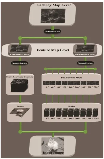
For an image , the model provides a global saliency value and a saliency map (Koch

& Ullman, 1985). The saliency estimation is achieved through the computation of orientation

and luminance Scales, which are then further combined to form Sub-Features Maps and

Feature Maps (see Figure 1). Since our saliency model is inspired by the one described in

Verma and McOwan (2009), only differences and crucial details of our approach are

discussed.

The model makes use of a hierarchical structure which was inspired by Marr’s (1982)

model of visual processing, and in particular, by the so-called primal sketch of a given visual

scene that employs feature extraction of basic components including regions, edges, textures,

etc. The outcome of the model can be defined as:

is the saliency model that returns two main outputs: , a global saliency value

estimated on the basis of the saliency map (i.e., ) obtained from a given image .

represents the weighting function used to combine maps at each step as depicted in

Figure 1 (see section 2.3). is the luminance channel and relates to the

channel that comprises 9 orientational filters. No colour channels are implemented as only

greyscale pictures were used.

The following two sections illustrate how luminance and orientation features are

extracted and then combined to form the saliency map and to compute its numerical

estimation.

2.1 Extraction of visually low-level information

Luminance

For the feature extraction we chose the implementation of a biologically inspired

centre-surround filter for luminance (Hubel & Wiesel, 1962). This involves obtaining a

Gaussian Pyramid of the image of interest (Burt & Adelson, 1983) and creating contrasts

according to a given rule (i.e. inter-scale subtraction; see Itti, Koch, & Niebur, 1998). The

construction of the pyramid starts from the original greyscale image. This scaling technique is

used to simulate centre-surround receptive fields in neuro-computational modelling and has

resulted in reasonably successful modelling of on/off simple receptive fields with a

Difference in Gaussian function (DoG) (Field & Tolhurst, 1986; Jones & Palmer, 1987; Marr

& Hildreth, 1980). This method is grounded in the assumption that simple cells in the visual

cortex V1 are sensitive to visual features that pop out against a homogenous background, e.g.,

when a foreground elicits a different neural activity compared to the background (Knierim &

van Essen, 1992; Nothdurft, Gallant, &Van Essen, 1999).

In order to build centre-surround filters we used the MatLab™ function impyramid

of a 2-dimensional Gaussian kernel to subsample the image in n scales by applying a scaling

factor of 2 (i.e. scales are progressively smaller copies of the same image), resulting in the

resolution of the image at the top of the pyramid being of its original dimension. To

determine the number of scales we applied the following formula:

[ ] (Equation 2)

and are the width and height of the input image . We used a 1000 1000 pixel

resolution to build images; this led to a constant number of scales (i.e., ). To allow

inter-scale subtractions among the previously obtained inter-scales, the down-sampled images were

resized to the original size using bilinear interpolation (see ‘scales’ and ‘centre-surround

contrasts’ in Figure 1). The number and the type of subtractions performed are based on the

following formulae:

(Equation 3)

where (Equation 4)

Because the number of Scales is equal to 7, we obtained a total of 9 luminance

contrasts, as follows: .

Orientation

The implementation of orientational filters cannot be successfully achieved by

standard DoG filters for several issues. One main problem is that that the orientation features

are more complex than those of uniform foregrounds or backgrounds, because the receptive

& Jessell, 2000). A log-Gabor filter is more suitable to model this computational aspect

(Valois, Albrecht, & Thorell, 1982).

A Log-Gabor filter is made from two components: a radial part (Fr) and an angular

part (Fa). The former defines the spatial frequency that the filter is sensitive to, whereas the

latter adjusts a periodic wave to the filter. This can be formulated as follows:

[ ( )] [ ( )]

(Equation 5)

_{(Equation 6)}

represents the orientation that the filter is selective to, is the centre of the

frequency domain, whereas and are respectively the bandwidths of the radial and

angular parts (measured in octaves). To avoid overlap between filters being selective to

different orientations, the ratio between the bandwidth of the radial part and the centre

frequency of filter is held constant.

The radial part is split into seven Scales (labelled 1 to 7). That is performed for all

nine orientation filters used in our implementation:

and . The higher number of orientation filters should enhance the performance of the

model compared to the Verma and McOwan (2009) implementation, where four filters were

used1.

1

The function used to compute Log-Gabor filters was scripted by Kovesi (2001, 2010) and available from the author’s website:

The two parts can be further combined to get the polar coordinates in the frequency

domain:

(Equation 7)

Following Valois, Albrect and Thorell (1982) the bandwidth was set to approximately

1.5 octaves, which is thought to be the norm to simulate orientation filters; whereas and

are respectively equal to 2 octaves and . For each orientation filter the wavelength is

set at 75Hz at the beginning (e.g. scale 1), and then reduced by a scaling factor of (with n =

1,…,7). Eventually the calculation of the orientation scales results in 63 scales (7 for each of

the 9 orientations).

2.2 Saliency Estimation

In order to quantify the amount of saliency present in a given image we utilised a peak

analysis approach according to the findings presented in Hu, Xie, Ma, Chia and Rajan (2004),

Verma and McOwan (2009) and Verma (2009). This is carried out for both the luminance

and orientation channels. The Hurst exponent estimation was implemented (Hurst, 1951;

Blok, 2000; Racine, 2011), which measures the amount of signal (i.e., quantifying the

saliency) present in a given map. Its value ranges between 0 and 1, approaching 1when the

map at issue contains a highly visible target-patch. This estimation can be achieved using

several methods (see Taqqu, Teverovsky, & Willinge, 1995). The Aggregated Variance

method (Taqqu et al., 1995) was chosen as this has the best trade-off between accuracy and

economy in terms of computational demand against the disadvantages of the methodologies

discussed in Hu, Xie, Ma, Chia, and Rajan (2004) and Li and May (2003). Moreover, this

approach appears to be biologically plausible in terms of sensory information analysed by the

To compute the Hurst estimation, pixels present in each shown in Figure 1 were

collapsed into two 1-dimensional data series. This was done by computing the standard

deviation of the image pixel values first by the x-dimension (i.e., pixel row) and then by the

y-dimension (i.e. pixel column). The two estimations are then summed to form a global Score

as follows:

( ) ( ) (Equation 8)

Where is the saliency value for a given , whereas and are

respectively the standard deviations of the data series computed on the x and y dimensions.

Since is the sum of two Hurst estimation, its range is from 0 to 2. When

approaches 2 there is a strong cross-correlation in terms of spatial similarity of the orientation

filter response across the data series. The main advantage of using the Hurst exponent is that

it favours isolated peaks against a series of peaks irrespective of the amplitude (e.g. low

frequencies against high frequencies; see Verma, 2009). The same applies to the luminance

contrasts. A single peak (e.g., a target-patch against a homogeneous background) is more

likely to be self-similar across a data series (e.g. having a low standard deviation), whereas

several peaks (e.g. a uniform background such as a target-absent image) determine a high

standard deviation and thus a lower is assigned.

2.3 Feature Combination

Combining scales, contrasts and maps is useful to reduce the number of maps per

feature being analysed, but maps containing higher amounts of signal need to be more

heavily weighted than others. Several methods are available to combine different scales and

contrasts (Itti & Koch, 2001; Verma & McOwan, 2009). A review of these combination

Logarithmic combination strategy (PA-Log). According to Verma (2009), PA-Log is more

reliable than other methods because it picks up a smaller spread of false detections, in that

maps with the highest scores (e.g. a strong localised peak detecting one target) will be given

a much higher weight than those with the lowest scores (e.g. a uniform background).

In order to weigh heavily those maps with the highest scores, maps are sorted in

descending order, so that the highest weights are assigned to maps with the highest scores.

This is achieved with the formula:

₍

) (Equation 9)

Where M is the total number of maps to be combined: this equals to 9 for the

luminance centre-surround contrastsand 7for the orientation scales; see the maps in Figure 1

at the centre-surround and scale level. This value varies as the process of obtaining the final

saliency map proceeds. For example, M = 2 at the feature map level (see Figure 1 at the

feature map level box). The symbol in Equation 9 represents the -th position that a given

sub-map occupies when they are sorted according to their scores.

When weights are obtained the following strategy is used to form a map that

combines different sub-maps:

∑ (Equation 10)

Where the -th represents the map to be combined (e.g. from the

sub-map with the strongest signal to the one with the weakest); whereas is the corresponding

weight according to the sorted scores (i.e. from the highest to lowest).

We normalised the newly generated maps to the range [ ]. A linear normalisation

(Equation 11)

Where is a newly produced map resulting from the combination of those

present at a lower level. Normalisation is an efficient method to overcome two potential

issues related to the estimation of the saliency. Firstly, the use of two different methods to

obtain the saliency present in the luminance and orientation channel (i.e., centre-surround

contrasts and log-gabor filters), may favour one feature over another. Secondly, the weighting

function produces overpowered pixels (i.e., outside the range [ ]) that need to be rescaled

to within [ ] without altering the result of the weighting process.

Normalisation takes place when luminance centre-surround contrasts and orientation

filters are combined to form respectively one luminance feature map and one single

orientation map, and again to obtain the final saliency map. Figure 1gives an illustration of

the normalisation points.

Several estimations can be computed in order to obtain the global saliency score for

the final saliency map (see top of Figure 1). However, according to Verma (2009) the best

estimate for the saliency is the sum of the maximum scores obtained from both luminance

centre-surround contrasts and orientational scales:

(∑ ) (Equation 12)

Where is the -th maximum saliency score obtained from one of the

9 orientation piles at scale level (bottom right of Figure 1); whereas isthe

to range between 0 and 20 for a 9 orientation filter model, and between 0 and 10

for a 4 orientation model (see later in Study 2 for a comparison between these two saliency

models).

The next section explains how the saliency model and its two main outputs, i.e. the

final saliency map and its numerical estimation are embedded into a Genetic Algorithm (GA)

used to produce pop-out pictures.

2.4 The Genetic Algorithm

A genetic algorithm (GA) is a function that uses several variables to find a solution or

group of solutions that maximise or minimise some quantity. It does this through a process

akin to reproduction and a fitnessfunction. Over time unfit individuals tend not to pass on to

the next generation whereas fitter individuals reproduce and pass on their traits to future

generations (Holland, 1975; Goldberg, 1989; De Jong, 1975; Koza, 1990). The fitness

function is the crucial aspect allowing evolution to take place over generations. In our

implementation the saliency model was used as a fitness function within a GA operating over

image stimuli. This allows an artificial process of selection to be performed to achieve

different levels of saliency for unbiased stimuli (from a minimum to a maximum level of

saliency). To create these stimuli we used a form of “Biomorph” based on the work of

Richard Dawkins presented in his book The Blind Watchmaker (1986).

In contrast to Dawkins, we avoided the use of the symmetry to prevent our artificially

generated stimuli from appearing to be related to real life stimuli and therefore we called

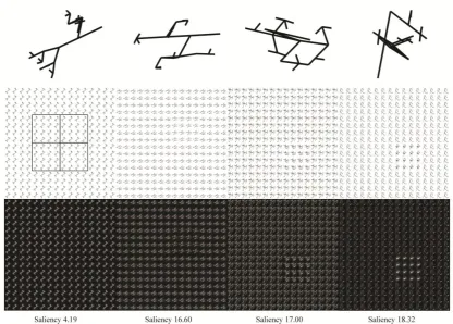
Figure 2. Top panel: four different randmorphs created in our implementation and used to produce a target-patch. Mid panel: one target-absent and three target-present patches at several levels of saliency. Left image shows a grid with the four possible positions for the target-patch. Bottom panel: the saliency maps obtained by the run of the saliency model with their saliency values given below.

Both our Randmorphs and Verma’s Biomorphs are a form of texton, fundamental

elements in visual perception that are used to form texture segregation images (Julesz, 1981;

Bergen & Julesz, 1983; Julesz, Gilbert, &Victor, 1978).

The GA in this implementation is a complex function that takes as an input several

components to give one output, which is a population of increasingly more salient pictures:

Where is the population bin: is the saliency model as described earlier

in the previous section, the set of centred coordinates for the target-patch, a

random parameter used to select the orientation of the branches for the randmorphs to be

drawn (see further), and the chromosome that stores the information for the drawing

of a pair of two randmorphs.

In order to operate the selection process we used both binary and integer encoding to

encode the chromosomes (Holland, 1975; Chakraborty, 2010; Davis & Mitchell, 1991;

Goldberg, 1989). A binary “genotype” chromosome consisting of 282-bits is employed to

express a pair of Randmorphs used to build a target patch image. Genes codify for integers

representing radians in the continuum between 0 and (rather than the range 0-2 ).

Simulations of the GA show that more occurrences of the same cosine and sine values for a

given radian lead to a smoother spread of the saliency values across the generations (see

Figure 3). To draw a pair of randmorphs a radian ( ) rounded to its nearest integer is

randomly selected to obtain 8 different orientations separated by an arbitrary unit of .

However, for simplicity, a set of orientations in degrees, rather than radians, is used to draw a

Figure 3. A wider range in the radian space was used to obtain more occurrences of the same cosine and sine values for a given radian (i.e., 57.32 ; see part A). For instance, (i.e. Z is a set of positive integer numbers including zero). This allows the drawing algorithm to build a broader range of randmorphs that leads the selection process to an evenly distributed continuum of saliency values, preventing the algorithm from producing sudden changes to the structure of the randmorphs (i.e. a smoother increase of the pop-out effect across images; see part B).

A “phenotype” chromosome is obtained from the 282-bit chromosome to form a

94-integer positions sequence, with each 94-integer represented by 3 bits and having a value ranging

between 1 and 8. Each phenotype chromosome is divided into two halves, each containing 5

segments coding for the following: first and second set of angles used to draw the two parts

of a randmorph (8 int. each), trunk of the randmorph (1 int.), left and right part of the

randmorph (respectively 15 int. positions; see Figure 4b and 4c). To draw a target-patch, a set

of centred coordinates in a 4 4 block lattice are randomly produced (i.e., ). Each

lattice block allows 16 replications of a randmorph. One randmorph is assigned as target and

reproduced 16 times to fill 1 out of 4 blocks surrounding the central area of the image (see

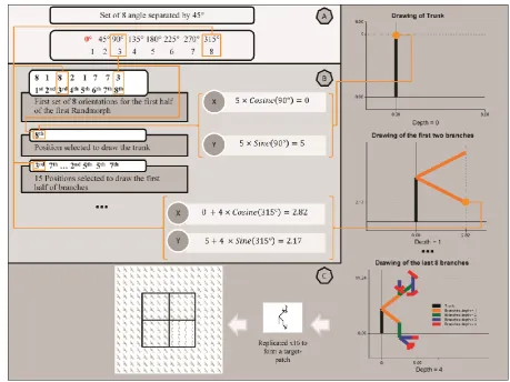
Figure 4. Part A: an angle is selected randomly to obtain a set of 8 angles separated by 45 degrees. For simplicity, we show here the drawing of a randmorphs in degrees (rather than radians). Part B: depicts the first 3 genome segments (out of 5) to construct the trunk and the first branch of the first half for the randmorph used as the target in the pop-out image. The first 8 genes codify the 8 orientation utilised to draw the first randmorphs. The next single-gene and the 15 that follow represent the positions of the angles selected in the first 8-integers sequence. Please note that this encryption allows two different loci to code for the same orientation. This allows branches to overlap and therefore to obtain a wide variety of patterns. Once the angle position has been retrieved from the chromosome, its corresponding angle is used to obtain the coordinates for the first segment to be drawn (trunk); this is done using cosine and sine functions. A scaling factor for the depth of the drawing is used to limit the pattern from getting too complex (starting from 5, i.e. depth = 0; see part C). Part C: represents the building of a randmorph by the drawing algorithm. Randmorphs are drawn in a two-dimensional space, with the first coordinate being (0,0). The drawing algorithm uses a recursive rule which diminishes the length of each segment by a factor of 1 at each depth. The final end of each segment is the starting point for the next two branches until the algorithm “runs out” at depth =4. Once the pair of randmorphs has been produced, one randmorph is used to construct the target-patch and therefore is replicated 16 times to form a square. A 4x4 lattice, each consisting of 16 positions, is used to form the image. The target-patch is allocated to 1 of 4 central positions. Overall, 256 randmorphs are used to produce a picture (240 to form the background plus 16 to create the target-patch).

Once the image has been obtained, a saliency map and a global saliency value are

produced by the fitness function (i.e., the saliency model); this provides the GA with the

The GA starts with a population of 12 images that is produced by the process

described above. An elitism approach was used (De Jong, 1975), which allows the fittest

images to be transferred to the next generation. This parameter was set to 0.2 which implies

that in our population of 12 individuals, 2 are selected as the fittest and passed on (e.g.,

individuals/images with the highest saliency values); whereas, the two least fit individuals in

the population are selected and passed on after the mutation function has applied a random bit

change. The mutation function changes the structure of the two binary chromosomes from

this starting population (the bit change probability is equal to 0.5)2. The first bit change is

always applied at depth = 4, proceeding through the generations towards depth = 0 (i.e., trunk

level) where a change usually determines a substantial change in the saliency of the image.

3

Studies

Two studies were performed to investigate differences between IB and non-IB

individuals in detecting the presence/absence of a target-patch on a uniform background. The

performance of the model will be also discussed.

Subjects in the two studies were classified as IB or non-IB on the basis of their

performance on a dynamic IB Task. In addition, the Randmorphs task was performed in the

two studies where the maximum stimulus exposure duration was 10s (Study 1) and 1s (Study

2). The model used to produce the saliency estimations in Study 1 was implemented with 9

orientational filters. Study 2 compared the performance of the 9 orientational filters model

2 _{The model does not make use of a crossover function. This is because in our implementation}

with a 4 orientational filters model, the latter being theoretically equivalent to the one

presented in Verma and McOwan (2009).

3.1 Study 1: 10-seconds Randmorphs task

We used a sample of 250 target-present images, along with an equal number of null

trials depicting a uniform texture of Randmorphs (i.e., target-absent). The goal was to

evaluate whether this model produced a reliable saliency estimate which allows predicting

human behaviour in terms of RTs to detect target-patches, and therefore discriminate between

IB and non-IB individuals.

In Study 1 the Randmorphs Task required participants to decide whether a target

region was present or not in each of the images. Each image had a saliency score as obtained

from the procedure outlined above. It was hypothesised that the time taken to respond to each

image would be negatively correlated with the saliency scores.

3.1.1 Apparatus

For the Randmorphs task stimulus images were presented on a 19-inch standard LCD

monitor (Samsung Sync Master 931BF) with a spatial resolution of 1280 1024 pixels and a

temporal resolution of 75Hz. Participants viewed the presented stimuli at a viewing distance

of 57 cm. The dimensions of the active display area were 33.9 27.1 cm. A chin rest was

used to constrain head movements. Subjects responded to stimuli using the Eprime S-R box.

The size of each stimulus image was 10.6 10.6 cm (378 378 pixels), so each image

subtended 10.6o of visual angle. Eye movements were monitored using an LC Technologies

video eye tracker with Eprime 2.0 (Schneider, Eschman, & Zuccolotto, 2002).

The same setting was used for the IB standard task apart from the following changes:

3.1.2 Participants

Twenty-five undergraduate students (3 male) from the Birkbeck College took part in

the study for course credit. The participants were naive about the purpose of the research. All

subjects had normal or corrected-to-normal vision and were aged 18 to 51 (mean=31.46;

SD=8.74).

3.1.3 Stimuli

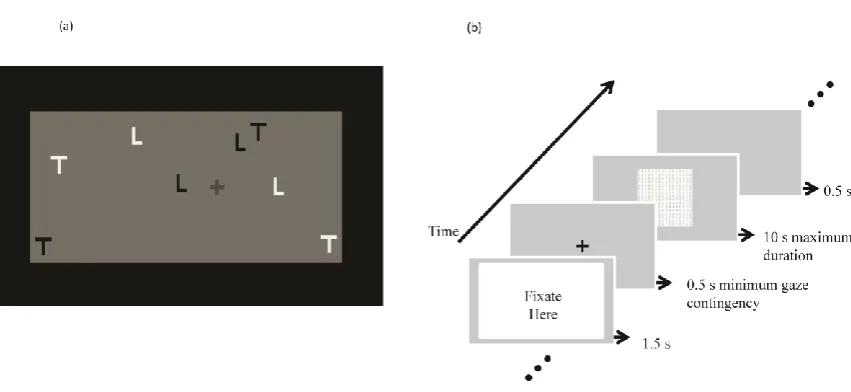
The IB Task (Figure 5a) was created using MatLab,and was very similar to the

dynamic IB task developed by Most et al. (2001; based on the video clip courtesy of Simons,

2003). The IB task comprised black and white letters (Ls and Ts) on a grey background

moving around the screen hitting the borders of the display. When the video begins there is a

still frame for 8.5 s showing the starting positions of the targets (white letters) and distractors

(black letters).

The primary task required that participants track the targets but ignore the distractors,

and report the number of times the targets bounced off the border of the display (i.e., ‘hits’) at

the end of the 32.5 s video. After 20 s from the onset of the video a red cross (in dark grey in

Figure 5a) moves across the screen, taking 11 s to traverse the screen starting from the right

hand side and exiting at the left side. Participants who failed to notice the red cross when

questioned at the end of the video were classified as IB subjects, whereas those noticing the

red cross as non-IB.

The randmorphs task consisted of 500 images, 250 of which were target-present

images. Each image display comprised a 4 4 grid. In 250 displays, one texton was

presented in each of these 16 positions, creating a seamless uniform background (i.e., target

absent displays). In the other 250 displays, one texton was used as the background (15

positions) but one of the four grid positions surrounding the central point was filled by a

second texton that served as the target (i.e., target-present). For the target-absent displays,

the saliency of the display ranged between 1.80 and 4.40 whereas for the target-present

displays, the saliency ranged between 11.79 and 18.20.

3.1.4 Procedure

Participants first completed the Randmorph task. Following the calibration procedure,

participants were instructed to view each display and to decide if there was a target present or

absent by pressing one of two keys on the response box. At the beginning of each trial a

screen displaying ‘Fixate Here’ was presented for 1.5 s. A gaze-contingent procedure was

then employed such that participants were required to maintain a central fixation for an

additional 500ms during which a fixation cross was displayed prior to the onset of the image.

This was implemented to standardise the starting position of the participants' fixation at the

asked to perform a 1 interval forced choice (1IFC) deciding whether or not a target region

was present (see Figure 5b). Participants were told they could freely look around from the

onset of the image and make a response anytime within the 10 s limit. Once the participant

has made a response, a 500 ms blank screen was presented before the beginning of the next

trial.

Participants were then presented with the IB task. They were instructed to silently

count the number of times the moving targets (white Ls and Ts) hit the border of the display

whilst ignoring the moving distractors (black Ls and Ts) – this was the primary task. At the

end of the task, participants were asked how many target hits they had counted and then

asked if they had seen anything else. Those participants reporting having seen the red cross

were classified as being non-IB whereas those who did not report it were classified as IB. All

participants who were classified as IB spontaneously reported seeing the red cross when they

were shown the task again but this time instructed not to do the counting task (i.e., full

attention task).

3.1.5 Results

The time taken to detect the target in the target-present trials was correlated with the

saliency level of the 250 trials (collapsed over all participants; IB status was not considered).

This showed a significant Spearman’s rho coefficient between the estimated saliency values

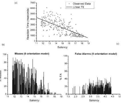
and reaction times (rs(248) = -.687; p<.001; one-tailed; see Figure 6a).

In addition, the same pattern is present if we consider the number of misses as a

function of saliency. As Figure 6b shows, the number of misses drops as the level of saliency

increases (rs(248) = -.736; p<.001; one-tailed). Interestingly, the number of false alarms

increases as saliency gets higher (rs(248) = 0.136, p<.05; two-tailed), although this

more inclined to see a target patch as the saliency increases, even though this is not present

(see Figure 6c; note that the saliency range for target-absent images is much lower because

the saliency is simply based on a uniform background).

Figure 6. (a) Plot of the linear fit, irrespectively of the IB status. Reaction times were fitted as a function of the saliency estimation for the target-present patches. This clearly shows that as the saliency increases the time taken to recognise a target-patch is longer, whereas the subject response for low saliency pictures is, albeit variable, significantly slower. (b) Histogram of miss rates as a function of the saliency, showing a proportional decrease as the saliency increases. (c) Histogram of false alarm rates as a function of the saliency, depicting an equally distributed pattern.

A linear fit was carried out (see Figure 6a, dashed line) that accounted for 44.6% of

the total variability (F(1,248) = 199.449, p<.001; R2 =0.446), with the predictor ‘saliency’

With respect to Inattentional Blindness, 6 subjects were not-IB whereas the remaining

15 subjects were IB. Two subjects were excluded as they appeared not to perform the primary

task properly (e.g. less than 11 out of 21 hits); moreover, two more subjects had to be

excluded because it was unclear from their report whether or not they notice the unexpected

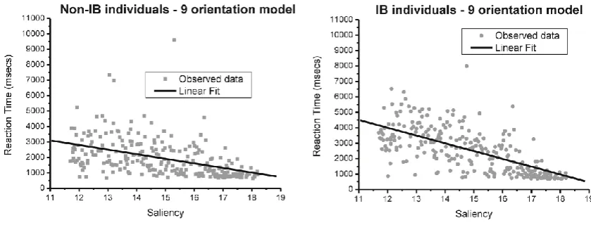
stimulus. Response times showed a different trend in the two groups. A multiple regression

with saliency and IB-status as predictors showed that the beta parameter saliency for the IB

group interpolates longer response times compared to the Non-IB group, with the latter

assumed as the baseline ( for dichotomous variable IB-status: = 0.934; t = 3.174, p<0.01;

see Figure 7). This was also confirmed from the negative estimate of the interaction term

(Saliency IB-status: = ; ): the regression line for IB

individuals, compared to Non-IB individuals, presents a more negative slope (i.e. inverse

relationship).

Figure 7. Linear fit for (left) non-IB individuals, and (right) IB individuals in study 1.

This shows that IB subjects are overall less sensitive to changes in the saliency of the

visual scene, whereas Non-IB individuals tend to pick up target-patches that are relatively

perform as quickly as Non-IB subjects (i.e., less sensitive). There was a significant

interaction between the two factors, and the addition of the interaction term increased the

amount of explained variance although only by 0.79 % ( ).

To evaluate saliency sensitivity differences between the two subgroups, was

calculated and an independent-samples t-test performed. Results show that although the two

samples present a different pattern for RT, the saliency difference are in the predicted

direction but not significant. The IB individuals are non-significantly poorer to identify a

signal among the noise ( , one-tailed; equal variances assumed;

̅ ̅ )3.

3.2 Study 2: one-second Randmorphs task

In order to check the replicability and generality of the findings of Study 1, a second

study was conducted using a shorter time window and so the presentation time for images

was reduced from 10 s to 1 s following by a 1 s blank interval. Participants were required to

respond within this shorter interval, which should reduce the influence of strategic processing

on performance. Secondly, we wanted to evaluate whether or not the removal of 5

orientational filters in the saliency model has an impact on the power of the model to

discriminate between IB and non-IB individuals. Thus a 4-orientational filters model

3

We also carried out the same analysis using more conservative criteria for the IB task (i.e., excluding those who counted less than 17 out of 21 hits or whose report was unclear). This resulted in the loss of 6 IB subjects whose performance was below the above criteria, although their report was clear. A t-test shows a difference in sensitivity ( ; two-tailed; equal variances assumed; ̅

(theoretically equivalent to the one present in Verma & McOwan, 2009), was compared with

the 9 orientation model.

3.2.1 Apparatus

The same experimental apparatus was used as for Study 1, but here the eye-tracker

was not used to monitor gaze contingent viewing. This is because a short presentation time

encourages participants to look at the centre of the screen as this is the most efficient strategy

(i.e., targets that appeared randomly in one of the four positions that surround this central

point are more likely to be detected if fixation is central rather than peripheral).

3.2.2 Participants

Twenty-nine subjects (9 males) took part in the study. All participants were naive

about the purpose of the research, had normal or corrected-to-normal vision and were aged

from 19 to 41 (mean=27.74; SD=6.02).

3.2.3 Stimuli

The saliency range was reduced because target-present images with the lowest

saliency values (e.g. 11-12) were too difficult to detect (an average of 55% of misses was

found in Study 1 between 11.70 and 13.00). Fifty-three target-present images in the

11.70-12.99 range were replaced with an equal number of new images evenly distributed along the

new range 13.00-18.70 for the 9 orientation model. The run of the 4 orientation filter model

on this modified image set gave a range of 3-10 for the same target-present images given as

input to the 9 orientation model. The same target-absent images used in Study 1 were utilised.

The saliency estimations from the 4 orientation filter model for these images ranged between

3.2.4 Procedure

The procedure remained the same as for Study 1 apart from reducing the duration of

image presentation. Subjects attended a screenshot showing a fixation cross for 2 s, followed

by a blank screen for 300 ms, and then the image appeared up to 1 s. Once the participant

made a response the image disappeared and a 1.5 s blank screen was presented before the

onset of the next trial. Responses were accepted within 2 s from the stimulus onset.

3.2.5 Results

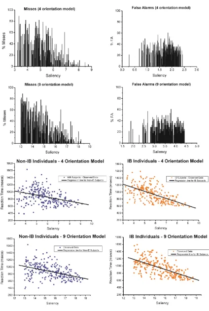
We compared the False Alarm (FA) rates for the target-absent images for the 9

orientation model here with those from Study 1, to evaluate the consistency of the saliency

values for the target-absent images across the two studies. Figure 6c and Figure 8a-b (right

panel) show that the FA rates follow the same pattern. We found no significant rho

correlations for both of the saliency estimations produced (4-filters model: rs(248) = -.08, p =

.205; two-tailed; 9-filters model: rs(248) = -.054, p = 0.39; two-tailed).

The saliency scores from the 4 orientation filter model showed a weaker correlation

(4-filters model: rs(248)= -.612, p<.001; one-tailed;) with target detection response latencies

compared to the ones from the 9 filter model (9 filter model: rs(248)= -.668, p<.001;

one-tailed; see Figure 8c and 8d). In order to compare the two correlations the Fisher’s r-to-z

transformation was utilised. Using the Fisher’s z-test (Howell, 1987), we found that the 9

filter model is not significantly better than the 4 filter model to predict participant’s reaction

times ( =1.06, p=0.146; one-tailed). However, an analysis of the misses showed

significant correlations with saliency for both models (4-filters model: rs(225)= -.717, p<.001

one-tailed; 9-filters model: rs(225)= -.790, p<.001; one-tailed), with the 9-filters model better

The goodness of fit of the two models was examined showing that, although both are

significant, they account for a different proportion of variance (4-filters model:

F(1,248)=139.500, p<.001, =0.360; 9-filters model: F(1,248)=193.525, p<.001;

=0.438). We then used a Cox test4 to compare the two non-nested models. Results from the

Cox test show that the two models are significantly different, with the 9-filters model

producing better saliency estimations when compared to the one with 4 filters only (

).

Fourteen participants were assigned to the IB group and seven to the non-IB group on

the same basis as for Study 1 (i.e., same exclusion criteria). No subjects were excluded on the

basis of the number of hits. However, 9 subjects were excluded as it was not possible to

determine whether they were inattentionally blind or not, as it was unclear from their reports

whether or not they noticed the unexpected stimuli (e.g., “something floating on the screen”,

“something red”, etc.). We therefore excluded these participants from further analysis.

A multiple regression with IB-status and the saliency estimations on RTs was

performed. Results show that IB subjects again were slower in detecting target patches

compared to the non-IB (4-filters model: IB-status: = 0.759; t = 4.24, p<0.001; 9-filters

model: IB-Status: = 1.412; t = 3.752, p<0.001). As for Study 1, we then included the

interaction term and we found it to be significant in both models (4-orientation model:

Saliency IB-status: = ; ; 9-orientation model: Saliency

IB-status: = ; ).

4

The inclusion of the interaction term in both models increased the proportion of

explained variance respectively of 1.7% for the 4 orientation model and 1.3% for the 9

orientation model (4 orientation model: ; 9 orientation model:

). However, there was a 6% difference in the amount of the

variance explained by the full 9 orientation model (main effect of saliency, group and their

interaction) when compared with the full 4 orientation model.

Because the two multiple regressions used to evaluate the saliency models are not

nested, we assessed which model produced a better estimation to predict the human

performance given the same number of regressors (i.e. the two main effects and their

interaction). A Cox test was again used to evaluate the two non-nested multiple regressions,

showing that the inclusion of the subjects’ status and its interaction with the regressor

‘saliency’ still favours the model with 9-filters ( ).

In summary, the addition of more orientational filters does increase the discriminatory

power of the 9 orientation filter model – compared to the 4-filters model – even for simple

images such as the ones that were used here (i.e., low-level images).

As for Study 1, we carried out a analysis between the two groups. No difference in

sensitivity was found in this study between IB and non-IB individual (

; one-tailed; equal variances assumed; ̅ ̅

)5.

5 _{This is also confirmed when we use a more conservative exclusion criteria, which led to the exclusion}

4

Discussion

The studies presented here show that the two models used to estimate saliency values

are able to pick up crucial visual details in the images used (e.g., luminance and orientation).

Changes in the pictures relate to the visual properties of the Randmorphs, and once the

structure of a pair of Randmorphs is sufficiently different, a human subject is able to detect

them as two separate entities on a screen. However, the saliency of the target patches was

estimated not only on the basis of the Randmorphs pair but also on the overall saliency scene

resulting from the replication of the pair throughout the lattice. This was done in order to

follow Gestaltic principles of perception (Von Ehrenfels, 1890; Koffka, 1935). It appears that

a target patch emerges from a higher-order pattern or gestalt, and the models presented here,

especially the one with 9 orientation filters, demonstrate that measuring this emergent

property may be possible. However, to test whether gestalts are leading to a pop-out effect, it

would be interesting to use pairs of Randmorphs of different saliency values in a visual

search task with varying set-sizes (targets and distractors previously used to form pop-out

images). This might give some insight into the strategies used by subjects: whether they are

using the saliency of the scene to identify the target, or they are performing a same-different

task. For instance, in our study we showed that performance is quicker when the saliency of

the image is high and the same number of target and distractors is used. This would suggest

an automatic processing at high saliency levels. However, set-size may play a role in

detection, inducing strategic processing when a small set-size is used (i.e., longer reaction

time; see for example: Schubö, Wykowska, & Müller, 2007; Schubö, Schröger, & Meinecke,

2004). In summary, it may be interesting to assess more closely the relationship between

The 9-filters model accounts for a significantly higher proportion of the variance than

the 4-filters model, even though this difference is small. However, it is likely that is due to

the low-level images utilised in the experiments, and that the difference would be more

pronounced if real-life images were used.

Furthermore, what is striking is that these visual features involve only low-level or

bottom-up properties and are sufficient on their own to provide a good prediction for how

long it takes for a human subject to identify patches on a monitor. This implies that

measuring the saliency may be carried out from the elementary constituents of a visual scene.

The importance of using this approach is that it prevents any possible confounding factors

from the manual selection or creation of images by the experimenter, which may introduce

top-down factors.

In order to reduce the influence of top-down processing, Study 2 reduced the

presentation of the images to 1 s. Even though the influence of strategic processing was

attenuated, we were still able to observe two different RT patterns for IB and non-IB subjects.

This supports the idea that not seeing something in a visual scene is influenced by low-level

factors (i.e., bottom-up). In an MEG study of working memory maintenance, van Dijk, van

der Werf, Mazaheri, Medendorp and Jensen (2010) found a modulation in the oscillatory

power, substantially in the alpha band of the posterior regions (but also in the beta), that

could be interpreted as a mechanism to inhibit task-irrelevant information (Klimesch, 1999;

Palva & Palva, 2007). When a stimulus (i.e., target patch) is processed, the alpha power

increases in those regions not necessary for the storage of information (Palva & Palva, 2007;

Jensen, Gelfand, Kounios, & Lisman, 2002). Conversely, finding no power modulation

(background alpha power remains unchanged or increases) during the presentation of a target

may be interpreted as an inhibition of the target from being processed. For instance, a low

robust level of saliency to allow this stimulus to be processed by the early attentional

mechanisms as sufficiently salient and therefore made accessible to consciousness.

However, this may not be the result of a low-level process. Some researchers argue

that that top-down factors may be influential when something is present but not noticed

(Dehaene & Changeux, 2005; Baluch & Ittti, 2011), and performance cannot be entirely

explained by low-level saliency factors (i.e., bottom-up factors) even when short durations

are used. The availability of a stimulus to awareness can depend on the state of the top-down

networks. For instance, Dehaene and Changeux (2005) showed in their model of

consciousness that the availability of a stimulus to awareness depends on the oscillatory

top-down activity, which can prevent the stimulus from being available to consciousness, even

though these stimuli have been processed to a lower level.

An EEG study may help to test this hypothesis, as a neural response can be observed

when the brain detects a target patch even when there is no associated behavioural response

(i.e., oscillatory top-down activity hindering the access of the stimulus to conscious

awareness). This may correlate with a decrease in the alpha power during the stimulus

presentation, showing that the stimulus has been processed at an early stage (Van Dijk et al.,

2010). Because we can quantify the saliency, we are able to give an estimate of the amount of

“salient” information necessary for the visual system to detect a target patch.

When a stimulus is processed at a low-level, high-level activity (mainly intrinsic

oscillatory activity in the gamma band) among cortical neurons can “ignite” a spontaneous

activity that can block external sensory stimuli from being available to awareness (Dehaene

& Changeux, 2005). This “covertly-processed-but-not-overtly-available-to-consciousness”

dissociation may explain why, for example, the same stimulus can be processed but not

activity. The images produced with our approach may be useful to further investigate this

phenomenon as they provide an easy way to measure the threshold for which a visual

unbiased stimulus is detected but not consciously available to the subject.

The models presented in this paper do not take into account the inter-element spacing

in the lattice (Julesz, 1981; Reddy & VanRullen, 2007; Franconeri, Jonathan, & Scimeca,

2010). Although this was addressed implicitly via the estimation of the Hurst exponent, there

is no modelling of such an attribute from which the models would benefit. This also applies

to the implementation of those mechanisms that evaluate the size, spatial distribution and the

density of elements in a visual scene (for instance bigger objects should have a higher

saliency and so on) 6. In addition, as the model used here is a low-level one, the modelling of

high-level factors (Baluch & Itti, 2011), may be beneficial to obtain a better saliency

estimation; this is particularly important for real life images, when the impact of semantics is

deemed to have a stronger effect (see for example the recent advances in computer science on

this point: Borji, Sihite, & Itti, in press). The two saliency models in the present paper are

likely to have performed better had real-life images been used rather than artificial

Randmorphs. Real-life images are by definition more complex and therefore the use of

additional orientational filters would help to discriminate small differences in saliency of the

scenes.

The amount of information picked up by the model is computed via the Hurst

exponent estimation, and one conspicuous limitation of this approach, for instance, is that one

target (e.g., single peak) is weighted more heavily than two targets (e.g. two similar peaks in

the same image; see Verma, 2009). As Verma (2009) suggests “a display with one red target

6 _{In our model there are no specific mechanisms to evaluate these visual features separately. The Hurst}

amongst a series of green targets produces a higher saliency value than a display with a group

of red targets amongst a background of green targets” (p.73). This means that a bias is present

only if we compare the saliency of two images with a different number of targets (e.g., one

with one target and one with two targets), whereas in the case of two images with the same

number of targets (e.g., one target each) the model is able to evenly estimate the saliency.

In summary, the approach presented here has demonstrated its accuracy in predicting

human performance under the condition of a visual pop-out search and has provided the

groundwork for this methodology to be used in the study of psychological processes such as

Inattentional Blindness. We have shown that IB subjects are on average slower than non-IBs

to detect targets on uniform backgrounds. However, previous research (e.g., Richards,

Hannon,Vohra, & Golan, 2013) has shown that this classification is affected by the visual

features of the paradigm, the primary task and the ability to cope with the cognitive demands

of the task . For example, in both studies reported here we used an IB Task that was very

similar to the one developed by Simons (2003). One possible issue with this standard IB task

is that the status of the unexpected stimulus is ambiguous. It does not form part of the

primary goal of the task, which is to count white targets and ignore black distractors, and it is

therefore not clear whether the most efficient or best strategy is to process the red cross and

remember it or to ignore it by either not processing it or by processing it and inhibiting it to

prevent it from interfering with the primary task (Richards, Hannon, Vohra, & Golan, 2013).

Previous research has shown that IB individuals, who typically have low working memory

resources, spend more time fixating irrelevant distractor stimuli compared to non-IB

individuals (e.g., Richards, Hannon, & Vitkovitch, 2010). One could argue that IB subjects

are less efficient than non-IB subjects just because they spend too much time looking at

irrelevant objects (i.e. not part of the primary task), and that training may be required for the

on a subsequent IB task (Richards, Hannon, & Derakshan, 2010; Richards et al., 2013).

Moreover, different types of IB tasks would inevitably produce different classifications. One

possible solution may be to use the saliency model on the visual aspects of the IB task in

order to manipulate their saliency and see how this affects the likelihood of noticing an

unexpected stimulus. Another interesting direction is to try to systematically investigate the

saliency difference necessary for IB subjects to perform as quickly as the Non-IB

subjects. This could be done by selectively manipulating the saliency of the pictures until no

difference in terms of RT performance is found. The difference would then give the extra

amount of saliency necessary for IB subject to perceive and therefore perform as Non-IB

subjects.

Taken together these findings suggest that further research is necessary on those

aspects of the visual processing that have an influence on the behaviour of the observer and in

its turn on brain activity. Nevertheless, we acknowledge that further model developments,

such as the inclusion of high-level processing (i.e. top-down), are necessary to achieve a

better saliency estimation. However, our results show that Non-IB individuals are better able

than IB individuals to pick up the saliency of a visual scene which is based on a low-level

saliency estimation (i.e., purely bottom-up). Non-IB subjects appear to be less influenced by

the saliency, giving a quicker response throughout the entire saliency range; whereas IB

subjects present longer reaction times when the saliency of the images is relatively low. At

high saliency values, the difference between the two groups is minor, and both present a

5

Acknowledgements

We would like to thank Manuela Andolfi (Motion & Graphic Designer,

http://vimeo.com/manuelaandolfi, [email protected]) for her contribution to the

6

References

Baluch, F., & Itti, L. (2011). Mechanisms of top-down attention. Trends in

Neurosciences, 34(4), 210-224.

Baluch, F., & Itti, L. (2011). Mechanisms of top-down attention. Trends in

Neurosciences, 34(4), 210-224.

Bergen, J., & Julesz, B. (1983). Parallel versus serial processing in rapid pattern

discrimination. Nature, 303, 696-698.

Blok, H. J. (2000). On the nature of the stock market: Simulations and experiments.

PhD thesis, University of British Columbia.

Borji, A., Sihite, D. N., & Itti, L. (in press). What/Where to Look Next? Modeling

Top-down Visual Attention in Complex Interactive Environments. IEEE Transactions on

Systems, Man, and Cybernetics, Part A - Systems and Humans, pp. 1-16.

Burt, P. J., & Adelson, E. H. (1983). The Laplacian pyramid as a compact image

code. IEEE Transactions on Communications, COM-31(4):532-540.

Chabris, C. F., Weinberger, A., Fontaine, M., & Simons, D. J. (2011). You do not talk

about Fight Club if you do not notice Fight Club: Inattentional blindness for a simulated

real-world assault. I-Perception, 2, 150-153.

Chakraborty, R.C. (2010). Fundamentals of Genetic Algorithms. Lecture slides,

Technology (JUET), Guna. Online source:

http://www.myreaders.info/html/artificial_intelligence.html.

Davis, L. D., & Mitchell, M. (1991). Handbook of Genetic Algorithms. Van Nostrand

Reinhold, New York.

Dawkins, R. (1986). The Blind Watchmaker. Penguin Books, London.

De Jong, K. (1975). An Analysis of the Behavior of a Class of Genetic Adaptive

Systems. PhD thesis, University of Michigan, Ann Arbor, Michigan. Department of Computer

and Communication Sciences.

Dehaene, S., & Changeux J.-P. (2005). Ongoing Spontaneous Activity Controls

Access to Consciousness: A Neuronal Model for Inattentional Blindness. PLoS Biol 3(5):

e141. doi:10.1371/journal.pbio.0030141

Desimone, R., & Duncan, J. (1995). Neural mechanisms of selective visual attention.

Annual Review of Neuroscience, 18:193-222.

Driver, J. (2001). A selective review of selective attention research from the past

century. British Journal of Psychology 92, pp. 53-78.

Ehrenfels von C. (1890). Über Gestaltqualitäten. Vierteljahresschr. fürPhilosophie,

14, 249-292.

Field, D. J. (1987). Relations between the statistics of natural images and the response

properties of cortical cells. Journal Optical Society of America, A, 4, 2379–2394.

Field, D. J., & Tolhurst, D. J. (1986). The structure and symmetry of simple-cell

receptive-field profiles in the cat’s visual cortex. Proceedings of the Royal Society of London,

Franconeri, S. L., Jonathan, S. V., & Scimeca. J. M. (2010). Tracking multiple

objects is limited only by object spacing, not by speed, time, or capacity. Psychological

Science, 21(7): 920-5.

Goldberg, D. E. (1989). Genetic Algorithms in Search, Optimization, and Machine

Learning. Addison-Wesley Longman Publishing Co., Inc., Boston, MA, USA.

Greene, W. H. (1993), Econometric Analysis, 2nd ed. Macmillan Publishing

Company, New York.

Greene, W. H. (2003). Econometric Analysis, 5th ed. New Jersey, Prentice Hall.

Hannon, E. M., & Richards, A. (2010). Is inattentional blindness related to individual

differences in visual working memory capacity or executive control functioning? Perception,

39, 309-319.

Holland, J. H. (1975). Adaptation in natural and artificial systems. University of

Michigan Press, Ann Arbor.

Howell, D. C. (1987). Statistical Methods for Psychology. Second edition. PWS

Publishers; revised Edition of 1st Edition 1982 edition. Duxury Press: Boston.

Hu, Y., Xie, X., Ma, W.-Y., Chia, L.-T., & Rajan, D. (2004). Salient region detection

using weighted feature maps based on the human visual attention model. Advances in

Multimedia Information Processing - PCM 2004, pages 993-1000.

Hubel, D. H., & Wiesel, T. N. (1962). Receptive fields, binocular interaction and

functional architecture in the cat’s visual cortex. Journal of Physiology, 160, 106–154.

Hurst, H. (1951). Long-term storage in reservoirs. Transactions of the American

Itti, L., & Baldi, P. (2008). Bayesian surprise attracts human attention. Vision

Research, Volume 49(10), pp. 1295–1306.

Itti, L., & Koch, C. (2001). Computational modelling of visual attention. Nature

Reviews Neuroscience, 2(3):194-203.

Itti, L., Koch, C., & Niebur, E. (1998). A Model of Saliency-Based Visual Attention

for Rapid Scene Analysis. IEEE Transactions on Pattern Analysis and Machine Intelligence,

20(11), 1254-1259.

Jensen, O., Gelfand, J., Kounios, J., Lisman, J.E. (2002) Oscillations in the alpha band

(9-12Hz) increase with memory load during retention in a short-term memory task. Cerebral

Cortex, 12, 877-882.

Jones, J. P., & Palmer, L. A. (1987). An evaluation of the two-dimensional Gabor

filter models of simple receptive fields in cat striate cortex. Journal of Neurophysiology, 58,

1233–1258.

Julesz, B. (1981). Textons, the elements of texture perception, and their interactions.

Nature, 290, 91–97.

Julesz, B., Gilbert, E. N., & Victor, J. D. (1978). Visual discrimination of textures

with identical third-order statistics. Biological Cybernetics, 31(14), 137-140.

Kandel, E. R., Schwartz, J. H., & Jessell, T. M. (2000). Principles of Neural Science.

McGraw-Hill Education.

Klimesch, W. (1999) EEG alpha and theta oscillations reflect cognitive and memory

Knierim, J. J., & van Essen, D. C. (1992). Neuronal responses to static texture

patterns in area V1 of the alert macaque monkey. Journal of Neurophysiology,

67(4):961-980.

Koch, C., & Ullman, S. (1985). Shifts in selective visual-attention towards the

underlying neural circuitry. Human Neurobiology, 4, 219–227.

Koene, A. R., & Zhaoping, L. (2007). Feature-specific interactions in salience from

combined feature contrasts: Evidence for a bottom-up saliency map in V1. Journal of Vision,

7(7:6): 1-14.

Koffka, K. (1935). Principles of Gestalt psychology. Oxford, England, Harcourt,

Brace.

Kovesi, P. (2010). Peter Kovesi Homepage. The university of western Australia.

Retrieved from http://www.csse.uwa.edu.au/~pk/Research/MatlabFns/index.html

Koza, J. R. (1990). Genetic programming: A paradigm for genetically breeding

populations of computer programs to solve problems. Technical report, Stanford University

Computer Science Department.

Kuhn, G., & Findlay, J. (2010). Misdirection, attention and awareness. Inattentional

blindness reveals temporal relationship between eye movements and visual awareness.

Quarterly Journal of Experimental Psychology, 63, 136-146.

Levin, D. T., Drivdahl, S. B., Momen, N., & Beck, M. R. (2002). False predictions

about the detectability of visual changes: The role of beliefs about attention, memory, and the

continuity of attended objects in causing change blindness. Consciousness and Cognition,