Global financial crisis and foreign development assistance shocks in least developing countries

Munich Personal RePEc Archive

Global financial crisis and foreign

development assistance shocks in least

developing countries

Das, Debasish Kumar and Dutta, Champa Bati

The University of Bonn

22 March 2012

Online at

https://mpra.ub.uni-muenchen.de/40281/

[1]

Global Financial Crisis and Foreign Development Assistance Shocks in

Least Developing Countries

Debasish Kumar Das

Department of Economics, The University of Bonn, Germany

Email: [email protected]/[email protected]

Champa Bati Dutta

Department of Economics, Khulna University, Bangladesh

Email: [email protected]

Abstract:

This paper evaluates whether the exogenous component of the global financial crisis affects

OECD-DAC EU donor countries ODA disbursements to the LDCs and how it impacts on LDCs economic

prosperity. Using both static and dynamic panel techniques, we find that global financial crisis in

OECD-EU donor countries are causes for the significant downside of ODA flows to the LDCs.

Consequently it adversely affects through the various transmission channels (e.g. ODA

disbursements, remittances, bilateral financial flows, export growth) to the LDCs economic growth.

Our results also explore that due to countercyclical role of ODA flows from the donors’ largely affect

to the LDCs economic development process negatively. The robustness checks using alternative

estimation technique supports our original estimation results in every context.

JEL Classification: O4, O5, O11, O19, F35, F39

[2]

1

Introduction

Foreign development assistance, widely known as Official Development Assistance (ODA), is the

most prominent development tool employed by the developed countries in its attempts to promote

prosperity in the developing countries. Since the Second World War, ODA has become an

institutionalized part of foreign policy of donors which accounts for an important source of many

developing countries’ fiscal income (Grant & Nijman, 1998). Several studies (Ang, 2010; C. Burnside

& Dollar, 2000; W. Easterly, 2003; William Easterly, Levine, & Roodman, 2004; Hansen & Tarp, 2001;

Karras, 2006; Rajan & Subramanian, 2005) have already widely explored the impact of ODA on the

Least Developed Countries’ (LDCs) economic growth. Some researchers have stated that ODA flows

also affects the foreign direct investment (FDI) inflows into developing countries, as donors always

encourage the improvement of the recipient countries’ FDI (Kimura & Todo, 2010; OECD, 2004).

Although the ODA’s impact on developing countries’ growth remains a subject for further

investigation, developing countries, in particular LDCs directly need foreign aid for their economic

development.

The recent financial crisis in the advanced economies has impacted LDCs heavily resulting in

reduced private financial flows and foreign aid, falling worker remittances and lower demand and

hence falling prices of the export goods. Consequently, these shocks have reduced LDCs income

growth rate by about 7 percent between 2007 and 2009 (Dang, Knack, & Rogers, 2009). Since LDCs

resources do not allow them to recover from these shocks by adopting fiscal stimulus packages like

the developed countries, ODA plays an important role to save them. In addition, ODA is mostly

connected with the development activities through some important sectors (e.g. infrastructure,

health, education, etc). Therefore, it is important to investigate whether the financial crisis has

affected ODA. If it proves to affect it then, it will be essential to investigate whether a sudden cut of

ODA disbursements will aggravate the problems already imposed by the crisis and further hinder the

[3]

(2005), Birdsall (2004), OECD (2003)and many others highlighted that volatility and

unpredictability of ODA shocks is a severe macroeconomic management problem to the LDCs.

There is a dearth of studies (Bulir & Hamann, 2008; Dang et al., 2009; Frot, 2009; Mendoza, Jones, &

Vergara, 2009; Minoiu, Zanna, & Dabla-Norris, 2010; Mold, Prizzon, Frot, & Santiso, 2010) that

examine the effects of the financial crisis on donor countries ODA flows. Dang et al. (2009) points

out that crisis affected donor countries have reduced their ODA flows by an average of 20 to 25

percent and bottom out only about a decade after the banking crisis; Roodman (2008), Frot (2009)

argue that the recent financial crisis will slump the ODA flows. This is supported by the reduction of

ODA disbursements following to the Nordic financial crisis in 1990’s. He reports that Nordic banking

crisis reduce donors’ aid disbursements by 13 percent. Conversely, Pallage and Robe (2001), Mold et

al. (2010) claims that the financial crisis and donor countries economic growth does not impact on

ODA disbursements and which may not have any negative impact on the developing economics.

However, the empirical evidences, methodologies and analyses of the above studies are not

sufficiently rigorous.

This research rigorously examines whether the exogenous component of the global financial crisis

affects OECD-DAC EU donor countries ODA disbursements to the LDCs and how it impacts on LDCs

economic prosperity. Methodologically, our research uses two econometric techniques: firstly, static

panel estimators and secondly, dynamic panel generalized method of moments (GMM) estimators.

We also run various specification tests to check the validity of the models and subsequently employ

the alternative econometric techniques to check the robustness of our models. We comprise various

yearly data for 17 OECD-DAC EU donor countries and 53 LDCs between 2004 and 2010. Our results

suggest that global financial crisis in OECD-EU donor countries declines their ODA effort to the LDCs.

Consequently it adversely affects through the various transmission channels (e.g. ODA

disbursements, remittances, bilateral financial flows, export growth) to the LDCs economic

[4]

The remainder of the dissertation is organized as follows: section 2 lays out the stylized facts of

global financial crisis and FDA shocks in least developing countries; section 3 presents data and

empirical strategy, while section 4 discuss and presents the static and dynamic panel estimation

results, and section 5 contains the conclusion.

2

Stylized facts

2.1

Global financial crisis and development assistance shocks

The current global financial crisis was initially triggered through the bursting of the United States

housing bubble in 2007. Soon after, in September 2008 the EU financial turmoil erupts and

contagion over the EU member countries, referred to is now as the so called global financial crisis.

Reinhart and Rogoff (2009) shows that, aftermath of this severe financial crises in rich countries

asset markets are collapsed and prolonged, output and employment level declines profoundly and

government debt tends to explode. Consequently, to mitigate and tackle the crises, OECD-DAC in

particular EU countries adopt the fiscal austerity measures, which are potentially affecting of their

ODA flows to the LDCs. Some donors have already cut their aid expenditure in terms of aid volumes1

and aid programming2 _{(te Velde & Massa, 2009), while OECD (2010)} estimates to meet the donors’

2010 ODA commitments at least 10-15 billion US$ must be added to their ODA spending plans.

1 _{e.g. Ireland by 24 percent, Italy 56 percent, Greece 32 percent, Denmark 11 percent and the Netherlands 11} percent.

[5]

Figure 2.1: Scenario of intensified financial stress in Euro area

[Source: IMF Economic outlook database]

Notes: This graph depicts the output gap, general government fiscal balance and general government lending/browning in the Euro area from 2004 to 2010 (from 2011 to 2015 is the IMF forecast). Evidence shows that the Euro area suffers deep economic recession from 2007 and onward, which is the causes of global financial crisis.

However, Sèna Kimm (2011), Jones (2011), Dang, Knack, and Rogers (2010), Faini (2006) explore

how the fiscal conditions of OECD donors affects their aid effort to the developing countries. They

finds that crisis affected donor countries reduce their aid flows by an average of 20 to 25 percent.

Additionally, they reports that aid flows is related to donors’ fiscal situation. Whereas Mendoza et al.

(2009) shows that financial and economic crisis has a negative link to the ODA disbursements by

using USA ODA disbursements from 1967-2007. Conversely, Mold et al. (2010) demonstrates crisis

does not impact on aid flows. Since limited numbers of studies have dealt with the supply side

perspective of donor ODA flows, these different empirical works did not sufficiently explore the real

picture of OECD-DAC ODA flows to the most ODA dependent low income counties after financial

crises, while they consider all OECD-DAC donors ODA flows to the developing countries (including

the emerging economies) as a whole. Therefore, there is no supporting evidence in this regard,

-7 -6 -5 -4 -3 -2 -1 0 1 2

04 05 06 07 08 09 10 11 12 13 14 15

General government net lending/borrowing

(Output gap,General government structural balance)

IMF Forecast

P

e

rc

e

n

ta

g

e

o

f

GD

P

[6]

which makes our research more essential. Here we consider only crisis affected regions’ OECD-DAC

donor countries and their supply side determinants of ODA disbursements only to the LDCs.

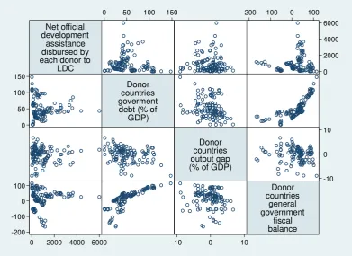
Figure 2.2: Scatter-plot matrix of OECD-DAC EU donors’ major economic indicators

Figure 2.2 exhibits a scatter-plot matrix of OECD-DAC EU donor countries major economic indicators

(e.g. ODA flows to the LDCs, public debt, output gap and government fiscal balance), which appears

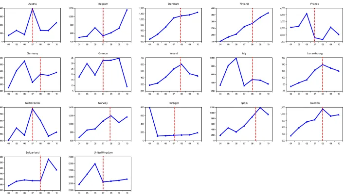
to show a strong relationship between these variables. Our figures3 _{(Figure 2.3) present the net ODA}

disbursements by the 17 OECD-EU donor countries to the 53 LDCs during pre and post financial

crises4_{. It clearly postulates that most of the OECD-EU} donors’ countries net ODA flows reduced

substantially since 2007, e.g. Austria, France, Germany, Ireland, Italy, Luxembourg, the Netherlands,

Norway, Portugal, Sweden and United Kingdom (UK). If we look before 2007, these EU donors’ net

ODA flows were gradually increased to the LDCs’ in terms of their commitments. According to

Reinhart and Rogoff (2009) evidence, our figures (see Appendix) show that the severe crisis affected

donor countries public debt and general government fiscal balance tend to explode since 2008.

3 _{Figures are computed by using the OECD-DAC database on net ODA disbursements by OECD-EU donor} countries to the LDCs, OECD-EU donors’ public debt and general government fiscal balance (see Appendix). 4 _{We use data from 2004 -2010.}

Net official development

assistance disbursed by each donor to

LDC

Donor countries goverment debt (% of

GDP)

Donor countries output gap (% of GDP)

Donor countries

general government

fiscal balance

0 2000 4000 6000

0 2000 4000 6000 0

50 100 150

0 50 100 150

-10 0 10

-10 0 10 -200

-100 0 100

[7]

Thus, our evidence demonstrates that before the crisis started EU donors net ODA flows to the LDCs

was consistent and upward with respect to their fiscal conditions but the following the crisis most of

[8]

Figure 2.3: OECD-EU donor countries net foreign development assistance disbursements to LDCs

0 100 200 300 400

04 05 06 07 08 09 10

Austria 400 600 800 1,000 1,200

04 05 06 07 08 09 10

Belgium 600 700 800 900 1,000 1,100 1,200

04 05 06 07 08 09 10

Denmark 150 200 250 300 350 400

04 05 06 07 08 09 10

Finland 1,500 2,000 2,500 3,000 3,500 4,000

04 05 06 07 08 09 10

France 1,000 1,500 2,000 2,500 3,000 3,500

04 05 06 07 08 09 10

Germany 5 10 15 20 25 30 35

04 05 06 07 08 09 10

Greece 200 300 400 500 600 700

04 05 06 07 08 09 10

Ireland 200 400 600 800 1,000

04 05 06 07 08 09 10

Italy 60 80 100 120 140 160

04 05 06 07 08 09 10

Luxembourg 1,300 1,400 1,500 1,600 1,700 1,800

04 05 06 07 08 09 10

Netherlands 600 800 1,000 1,200 1,400

04 05 06 07 08 09 10

Norway 0 200 400 600 800

04 05 06 07 08 09 10

Portugal 0 200 400 600 800 1,000 1,200

04 05 06 07 08 09 10

Spain 600 700 800 900 1,000 1,100

04 05 06 07 08 09 10

Sweden 300 350 400 450 500 550 600

04 05 06 07 08 09 10

Switzerland 2,000 3,000 4,000 5,000 6,000 7,000

04 05 06 07 08 09 10

[9]

2.2

Development assistance shocks and least developing countries

In the decade prior to the global financial catastrophe, bilateral ODA disbursements to the

developing countries consistently increased; as a result the crisis raised big concerns that ODA

supply would decline (Dang et al., 2009; Frot, 2009; Minoiu et al., 2010). However, developing

countries, in particular LDCs are now experiencing the magnitude of the global financial turmoil,

which hit hard primarily their private capital flows, ODA and remittances, trade revenue and many

others macroeconomic variables. These transmission channels primarily evolve through reduced

ODA disbursements, export growth, private capital flows and workers’ remittances flows to the

LDCs, which put them from frying pan into the fire. Consequently, these transmission mechanisms

have induced broad adverse macroeconomic effects to the LDC’s economy, for instance; growth,

investment, poverty, inequality, public and private debt and so on. Bulir and Hamann (2008)

demonstrates that aid dependent countries heavily suffer from the external shocks and due to the

widespread liquidity constraint they are less able to absorb those shocks.

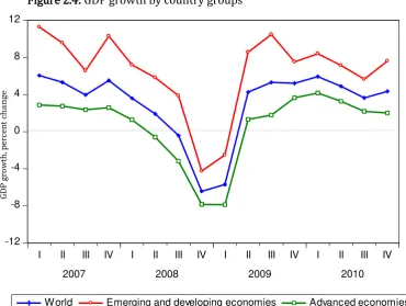
Figure 2.4: GDP growth by country groups

[Source: IMF World Economic Outlook database]

-12 -8 -4 0 4 8 12

I II III IV I II III IV I II III IV I II III IV

2007 2008 2009 2010

World Emerging and developing economies Advanced economies

GD

P

gr

o

w

th,

p

e

rc

e

n

t

c

hang

[10]

Notes: This graph reflects the quarterly GDP growth rate from 2007 to 2010 of global economies, emerging and developing economies and advanced economies. It shows that the financial crisis in advanced economies rapidly affects to the emerging and developing countries GDP growth rate through various transmission channels. Although developing countries, in particular the LDCs may not have played any role for this big recession, but they are severely affected through the global market actions.

Furthermore, ActionAid (2009) estimates that low income countries export growth decline almost

25 percent in side-by-side financial resources to around US$ 300 billion (Cali, Massa, & te Velde,

2008; Naudé & Research, 2009). Dang et al. (2009) show that developing countries income growth

rate is reduced by about 7 percent between 2007 and 2009. In terms of ODA, the Doha Monetary

Consensus meeting in 20085 _{revealed that most of the OECD-DAC donors could not meet their aid}

commitment6 _{to the developing countries (Cali et al., 2008; Naudé & Research, 2009). Subsequently,}

foreign direct investment (FDI) flows decreased by 10 percent in 2008 (UNCTAD, 2009) as well as

workers remittance flows being reduced considerably. Thus, it is obvious that developing countries,

particularly LDCs economic growth and development are in difficulty after the financial crisis and

economic recession of 2008 and 2009 in donor countries.

LDCs are already severely affected by the global financial crisis and additional ODA cuts put them

more miserable situations, where over 50 percent people lives under the poverty line7_{. Most}

importantly, LDCs are far behind to reach United Nations Millennium Development Goals (MDG) e.g.

poverty reduction, education, health, environment, economic growth and so on, thus ODA shocks

potentially a big threat to their development progress. Our figures (see Appendix) portray that the

LDCs’ (e.g. Bangladesh, Benin, Burundi, Cambodia, Central African Rep., Chad, Kenya, Haiti, Laos,

Lesotho, Liberia, Mali, Mauritania, Mozambique, Senegal, Sudan, Togo, Tajikistan, Vanuatu, Vietnam,

Yemen and so on) worker remittances, debt forgiveness reduction, export growth and bilateral

financial flows decline substantially since the financial crisis of EU donor countries, on the other

hand in this period most of the LDCs’ affected by different types of severe natural disaster as well.

5 _{OECD-DAC follows up international conference on financing for development to review the implementation of} the monetary consensus in Doha, Qatar, December 2008.

6 _{In 2002, monetary consensus on financing for development OECD-DAC donor countries have agreed to} provide at least 0.7 percent of their GNP as aid to the developing countries.

[11]

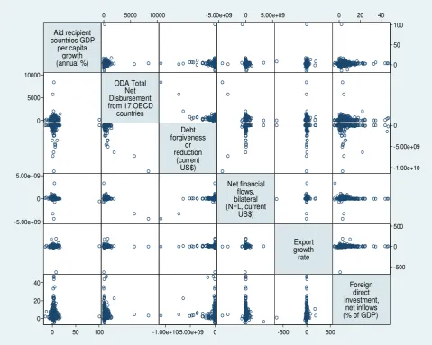
Moreover, Figure 2.5 presents a scatter-plot matrix of the LDCs’ per capita economic growth, net

ODA disbursements from OECD-DAC EU donor countries, debt forgiveness reduction, net bilateral

financial flows, export growth rate and foreign direct investments. This graph shows that net ODA

disbursements from OECD-DAC EU donor countries, debt forgiveness reduction, net bilateral

financial flows, export growth rate and foreign direct investments have a strong link with the LDCs

per capita economic growth. Thus this stylized fact confirms us to investigate how ODA and other

financial flows shock affect to the LDCs.

Figure 2.5: Scatter-plot matrix of the LDCs major economic indicators

2.3

Shortcomings of exiting examination

There is a few number of studies (Bulir & Hamann, 2008; Dang et al., 2009; Frot, 2009; Mendoza et

al., 2009; Minoiu et al., 2010; Mold et al., 2010) that account for the effects of the financial crisis on

Aid recipient countries GDP

per capita growth (annual %)

ODA Total Net Disbursement from 17 OECD

countries

Debt forgiveness

or reduction

(current US$)

Net financial flows, bilateral (NFL, current

US$)

Export growth rate

Foreign direct investment,

net inflows (% of GDP)

0 50 100

0 50 100 0

5000 10000

0 5000 10000

-1.00e+10 -5.00e+09 0

-1.00e+10-5.00e+09 0 -5.00e+09

0 5.00e+09

-5.00e+09 0 5.00e+09

-500 0 500

-500 0 500 0

20 40

[12]

donor countries ODA flows. However, the empirical evidences, methodologies and analyses of these

studies are not sufficiently rigorous. Roodman (2008) and Mold et al. (2010) study are more

discussion oriented and provides less empirical evidence regarding their hypotheses. Furthermore,

Roodman (2008) does not show any further analysis of ODA disbursements of donor countries after

the effects of Nordic financial crisis. Frot (2009) estimates panel data of donor countries using vector

autoregression (VAR) model. He mainly considers a long time series data along with banking crises

data, consequently the results do not exhibits the actual evidence of the recent global financial crisis.

Besides, they do not verify their specification using alternative estimations for robustness checks

and sensitivity of the results. Minoiu et al. (2010) and Dang et al. (2009) estimate panel data using

fixed effects estimation. The weakness of their paper is the credibility of specification as they only

employed fixed effects techniques. Since, endogeneity is a big issue for panel data analysis, they

ignores the necessary specification tests to examine the correlation between regressors and

unobserved country-specific effects. Moreover, they do not carried out any other estimation

techniques even for the robustness checks of their obtained specifications. Furthermore, Mendoza et

al. (2009) uses only U.S. ODA disbursements data (1967-2007) for their estimations and ignores the

other OECD donor countries, thus their results does not portrait the comprehensive effects on ODA

flows to the recipient countries. Most importantly, none of these researches account for the impact

of ODA shocks to the LDCs, where the world poorest people are living.

3

Data and Empirical strategy

To analyze these issues we employ a robust econometric technique which directly deals with the

potential biases induced by omitted variables, simultaneity and unobserved country specific effects.

Methodologically, we have used both static and dynamic generalized method of moment (GMM)

panel estimation procedure. To use these techniques we have set up two models: (1) for OECD-EU

donor countries and (2) for LDCs. We assemble the panel data set of 17 countries from donor

perspective and 53 countries from recipient perspective. To address the question concerning the

[13]

it is the per capita gross domestic product (GDP) growth. The explanatory variables of both model

contains a large set of variables which serves as conditioning information.

3.1

Data

We consider two panel data sets from the complementary points of view of the donor countries and

of the recipient countries. Our sample covers the period 2004-2010. For our first panel we limit

sources counties to the 17 OECD-DAC EU donor countries, since EU donor countries are severely

affected by the financial crisis. And for our second panel we limit sources to the 53 Least Developed

Countries, whose economic development is largely, depends upon Foreign Development Assistance

(FDA) received from donor countries.

3.1.1

Donor countries data

Our first hypothesis is to examine whether the exogenous component if the financial crisis affects

OECD-EU donor countries ODA disbursements to the LDCs. Data for OECD-EU donor countries are

taken from EuroStat, OECD-DAC, database8_{, which are the standard sources used in empirical}

research. Our data set represents strongly balanced panel of 119 observations and 17 countries for

the period 2004-2010 each.

We considered Net Official Developed Assistance (ODA) disbursement instead of ODA commitments

by each donor to the developing countries, as there was a wide gap between ODA commitments and

ODA disbursements by each donor in the data sets. For banking crisis data, we used a database

developed by Luc Leaven9_{. From this, we considered the banking crisis events after 2004, since most}

of the EU donor countries were affected by the financial crisis after this time period. We suspect

banking crisis in a donor country is one of the major channels to reduce the ODA disbursements

irrespective of its effect on the other macroeconomic variables. We also consider budget deficit and

public debt (DPD), output gap (DOG), general government fiscal balance (DGGFB), trade openness

(TOP), GDP per capita (GDPC), population (Pop), real effective exchange rate (RER), rate of inflation

[14]

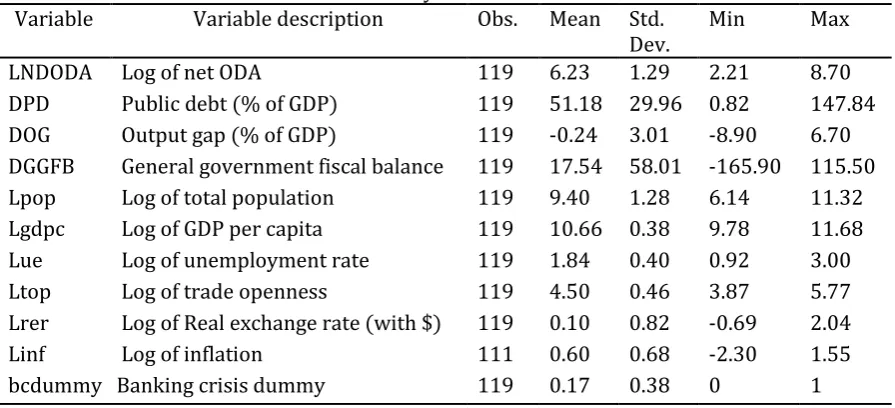
(INF) and rate of unemployment (UE) data, which are affect to the ODA flows to the LDCs. Table 3.1

represents summary statistics of OECD EU donor countries variables used in the estimation.

Table 3.1 OECD-EU donor countries summary statistics

Variable Variable description Obs. Mean Std.

Dev.

Min Max

LNDODA Log of net ODA 119 6.23 1.29 2.21 8.70

DPD Public debt (% of GDP) 119 51.18 29.96 0.82 147.84

DOG Output gap (% of GDP) 119 -0.24 3.01 -8.90 6.70

DGGFB General government fiscal balance 119 17.54 58.01 -165.90 115.50

Lpop Log of total population 119 9.40 1.28 6.14 11.32

Lgdpc Log of GDP per capita 119 10.66 0.38 9.78 11.68

Lue Log of unemployment rate 119 1.84 0.40 0.92 3.00

Ltop Log of trade openness 119 4.50 0.46 3.87 5.77

Lrer Log of Real exchange rate (with $) 119 0.10 0.82 -0.69 2.04

Linf Log of inflation 111 0.60 0.68 -2.30 1.55

bcdummy Banking crisis dummy 119 0.17 0.38 0 1

3.1.2

Developing countries data

To address our second research hypothesis- investigate how ODA and other financial flows shock

affect to the LDCs., we consider 53 Least Developing Countries (LDC)10_{. In fact, we restrict our}

attention only to the LDCs, since these world’s most poor cohort countries are facing several

challenges due to the global financial crisis, which include huge debt burden, very limited inflows of

FDI, low rate of ODA and remittance inflows, less participation in export and so on.

For our strongly balanced panel for 53 LDCs represents 371 observations for the time period

2004-2010. We used data from various sources, including the Penn World Tables 7.011 _{, OECD-DAC , Global}

Development Finance Report (2012), World

Bank, IMF-International Financial Statistics,

WIDER, ILO-Labor market statistics, Migration and Remittances

Emergency events database12_{. For this Panel dataset, GDP per capita growth rate treats as a}

dependent variable. We consider net total ODA flows rather than ODA commitments from the

10 _{Treated as low} income and lower middle income countries according to the World Bank’s classifications in 1990s.

11 _{See http://pwt.econ.upenn.edu/}

[15]

EU donor countries to the ODA recipient countries. Since, European Union (EU) member countries

are severely affected by global financial crisis, thus we also restrict our attention only to the

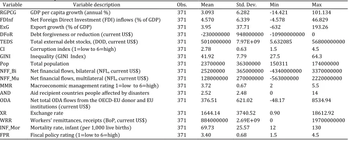
OECD-EU donor countries ODA flows. The other explanatory variables include net FDI inflows, export

growth, debt forgiveness or reduction, total external debt stocks, corruption index, inequality (GINI

index), total population, net bilateral financial flows, net multilateral financial flows, macroeconomic

management rating, numbers of natural disasters affected, exchange rate, workers’ remittances,

infant mortality rate and fiscal policy rating also taken into consideration, which serves as

[16]

Table 3.2LDCs summary statistics

Variable Variable description Obs. Mean Std. Dev. Min Max

RGPCG GDP per capita growth (annual %) 371 3.093 6.282 -14.421 101.134

FDInf Net Foreign Direct Investment (FDI) inflows (% of GDP) 371 4.570 6.339 -4.578 46.829

ExG Export growth (% of GDP) 371 3.95 37.71 -632 193.26

DFoR Debt forgiveness or reduction (current US$) 371 -230000000 948000000 -10900000000 0

TEDS Total external debt stocks, (DOD, current US$) 371 5010000000 7.97E+09 5.632085 56800000000

CI Corruption index (1=low to 6=high) 371 2.78 0.63 1.5 4.5

GINI Inequality (GINI Index) 371 41.92 7.79 27.5 64.3

Pop Total population 371 23700000 36300000 150311 174000000

NFF_Bi Net financial flows, bilateral (NFL, current US$) 371 25200000 365000000 -4340000000 3370000000

NFF_Mu Net financial flows, multilateral (NFL, current US$) 371 128000000 270000000 -563000000 2220000000

MMR Macroeconomic management rating 1=low to 6=high) 371 3.72 0.67 2 5.5

AND Aid recipient countries people affected by disasters 371 2.52 2.48 0 14

ODA Net total ODA flows from the OECD-EU donor and EU

institutions (current US$)

371 376.51 621.02 -48.17 8534.94

XR Exchange rate 371 1644.14 3740.52 0.90 18612.92

WRR Workers' remittances, receipts (BoP, current US$) 371 884000000 2.69E+09 0 19700000000

INF_Mor Mortality rate, infant (per 1,000 live births) 371 69.73 25.57 12 130

[17]

3.2

Empirical strategy

Considering the panel data, we would like to take into account how financial crisis within an

OECD-EU donor country may have an effect on country’s ODA disbursements to the LDCs over time. We

would also like to investigate how ODA flow shocks affect the LDCs’ economic development process.

To estimate the corresponding model, we employ two types of estimation techniques; static panel

estimation and dynamic Generalized Method of Moments (GMM) panel estimation.

3.2.1

Static panel estimation

We start with Pooled Ordinary Least Squares (POLS) estimation for our models. According to

econometric assumption, the OLS estimators are consistent when all explanatory variables are not

correlated with the error term. However, there is a possibility to violate this assumption if

explanatory variables are correlated with the error term and/or unobserved country specific effects

i.e. endogeneity problem.

Consider traditional cross-country regressions, our empirical models are as follows:

  '  

, , ,

lnNDODA_{i t} [ ]X _{i t i i t}

(1)

  '  

, [Z], ,

i t i t i i t

RGDPCG

(2)

Where, Eq. (1) and (2) represent 17 OECD-EU donor countries and 53 LDCs respectively. In Eq. 1,

lnNDODA is the logarithm of Net ODA disbursed by each donor considered as dependent variable

and X represents the set of explanatory variables (donor countries public debt, output gap, general

government fiscal balance, log of population, log of trade openness, log of real effective exchange

rate, log of inflation rate, log of unemployment rate and banking crisis dummy).



independently distributed error term with _, 0 and the subscripts i and t denotes country

and time period respectively. _iis an unobserved country specific effects which are not correlated

with



In Eq. (2), RGDPCG is the ODA recipient countries’ GDP per capita growth treated as a dependent

[18]

from each countries, net foreign direct investment inflow, debt forgiveness or reduction, total

external debt stocks, worker’s remittance, GINI index, export growth, corruption index, total

population, net bilateral financial flow, net multilateral financial flow, fiscal policy index,

macroeconomic management index, exchange rates, infant mortality rate and affected by natural

disaster). _iand



When we execute pooled OLS (POLS) regression, we do not consider unobserved country specific

effects for our models, Eq. (1) and (2). Thus, heterogeneity of the countries can appear of the

estimated parameters. As a result, we estimate the models incorporate unobserved country specific

effects by Fixed Effect (FE) and Random Effect (RE) techniques. However, incorporating the country

specific effects has several benefits, e.g. it allows accounting for specific effects. Later we use

Breusch and Pagan’s LM test to test the relevancy of unobservable country specific effects. This test

helps us to decide between RE and POLS. If we reject the null hypothesis13 _{POLS is not the}

appropriate technique for estimation and vice versa. Additionally, we also use the Hausman test14 _to

examine the correlation between regressors and unobserved country specific effects. The Hausman

test allows us to test for the misspecification between FE and RE estimation. Furthermore we

estimate FE and RE with AR (1) disturbance. To test for AR (1) disturbance we perform Baltagi-Wu

locally best invariant test. Since, several literature suspects the possibility of endogeneity of foreign

aid in the growth regressions (Alesina & Dollar, 2000; Boone, 1994, 1996; C. Burnside & Dollar,

2000; C. Burnside & Dollar, 2004; Hadjimichael, Ghur, Muhleisen, Nord, & Ucer, 1995; Hansen &

Tarp, 2001), we consider the endogeneity of ODA and employ Two-Stage Least Square (2SLS)

13 _H

0 : Irrelevance of unobserved country specific effects and HA : Relevance of unobserved country specific effects.

14 _H

[19]

technique for FE, RE and Baltagis’s Error Components 2SLS (EC2SLS15_{) RE estimator. Lastly, we use}

the Hausman test to compare these estimators’ results.

3.2.2

GMM estimators for dynamic panel models

Since, the static linear panel model does not permit us to analyze the possible dynamism, we use the

dynamic panel estimators that were pioneered by Holtz-Eakin, Newey, and Rosen (1988), Arellano

and Bond (1991), Arellano and Bover (1995), Blundell and Bond (1998) and Bond, Hoeffler, Temple,

and Research (2001). Our two panels consist of data from 7016 _{countries over the time period}

2004-2010. Since we use yearly data, our panel permits seven observations for each country. In dynamic

framework, Eq. (1) and (2) can be written in following specifications;

  _   

   '  

, 1 , 1 , ,

lnNDODA_{i t} lnNDODA_{i t} [ ]X _{i t i i t}

(3)

  _   

   '  

, 1 , 1 [Z], ,

i t i t i t i i t

RGDPCG RGDPCG

(4)

For

i

N

t

T

 

 

component structure;

For Eq. (3),

E



E



E

 

i

N

t

T





 

[ _i] 0, [ _{i t}] 0, [ _{i t i}] 0 for 1,... and 2,....

E

E

E

i

N

t

T

Now, we take the first difference to eliminate country specific effects of Eq. (3) and (4),

 







   





 











'

, , 1 1 , 1 , 2 , , 1

, , 1

ln

ln

(ln

ln

)

[

]

(

)

i t i t i t i t i t i t

i t i t

NDODA

NDODA

NDODA

NDODA

X

X

(5)

15 _{Baltagi (1984) shows Monte Carlo experiments on a two-Eq. simultaneous model with error components} and demonstrates the efficiency gains in terms of mean squared error in performing EC2SLS (see Baltagi 2005).

[20]

 







   





 











'

, , 1 1 , 1 , 2 , , 1

, , 1

(

)

[Z

Z

]

(

)

i t i t i t i t i t i t

i t i t

RGDPCG

RGDPCG

RGDPCG

RGDPCG

(6)

In the fact that for both Eq. (5) and (6), the lagged dependent variable (ln

NDODA



ln

NDODA

RGDPCG

RGDPCG





which implies that the regressors are likely endogenous. Thus, we need to use instruments to deal

with Eq. (5) and (6). According to econometric assumptions, the error term is not serially correlated

and the regressors are weakly exogenous17_{. Therefore, the dynamic panel GMM estimator employs}

the following moment conditions based on difference estimator for Eq. (3);





     

, , , 1

[ln _{i t s}( _{i t i t} )] 0 for 3,... , 2

E

NDODA

t

T

s





     

, , , 1

[ _{i t s}( _{i t i t} )] 0 for 3,... , 2

E X

t

T

s

Similarly for Eq. (4) is;





     

, , , 1

[ _{i t s}( _{i t i t} )] 0 for 3,... , 2

E RGDPCG

t

T

s





     

, , , 1

[ _{i t s}( _{i t i t} )] 0 for 3,... , 2

E Z

t

T

s

Which can be written in following matrix form as;

1

1 2

1 , 2

0 0 0 0

0 0 0

0 0 0

i

i i

i i T

y

y y

M

y y _

 

 

 

  

 

 

 

[21]

Here, M is the instruments matrix corresponding to the endogenous variables, where

y



,

ln

NDODA

RGDPCG

However, the first differenced estimator is criticized in terms of bias and imprecision. Thus, to

reduce potential biases and imprecision, Blundell and Bond (1998) suggest that, when regressors

have short time period, we can use a new estimator that combines a system in the difference

estimator with the estimator in levels, which is called the Blundell and Bond system GMM. The

difference operator in Eq. uses the same instrument as above and the instruments for the levels are

the lagged difference of the regressors. The econometric assumption here is that the difference in the

regressors and the country specific effect are uncorrelated. Therefore the stationary properties are:

For Eq. (3); E[lnNDODA_{i t p, } _i]E[lnNDODA_{i t q, }_i] and [E X_{i t p, } _i]E X[ _{i t q, }_i] p and q

The additional moment conditions for the levels are

 

 _,  _,  

[ ln _{i t s}( _{i i t})] 0 for 1

E

NDODA

s

 

 _,  _,  

[ _{i t s}( _{i i t})] 0 for 1

E

X

s

For Eq. (4);

E RGDPCG



E RGDPCG



E Z



E Z



m

n

The additional moment conditions for the levels are;

 

 _,  _,  

[ _{i t s}( _{i i t})] 0 for 1

E

RGDPCG

s

 

 _,  _,  

[ _{i t s}( _{i i t})] 0 for 1

E

Z

s

Now we can use GMM technique for both models to estimate consistent and efficient parameter by

employing the moment conditions given in Eq. (7), (8), (11) and (12) for the OECD-EU donor

[22]

Finally, to check the validity of the instruments in the system-GMM estimator, we implement two

specification test, which is suggested by Arellano and Bond (1991), Arellano and Bover (1995) and

Blundell and Bond (1998). First, the Sargan test of over-identification to check the validity of the

instruments and second the Arellano-Bond test to check the hypothesis that error term is serially

uncorrelated.

4

Estimation results and discussion

This section presents the estimation results of our research, which aims to answer our two prime

objectives: firstly, whether the exogenous component of the global financial crisis affects OECD-EU

donor countries ODA disbursements to the LDCs and secondly, how it impacts on LDCs economic

prosperity. We estimate Eq. (1) and (2) on the data set described above by using static panel

methods and Eq. (3) and (4) by using dynamic panel GMM estimation. We also run various

econometric tests to check the validity of our models plus the hypothesis of interest, and

subsequently discuss the robustness checks of our obtained estimation results.

4.1

Static panel estimation results

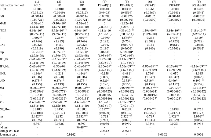
To analyze of our hypotheses, first we employ static panel estimation techniques in Eq. (1) and (2).

Tables 4.1 and 4.2 depict the estimation results of OECD-EU donor countries (Eq. 1) and LDCs (Eq. 2)

respectively. In both tables columns 1 to 8 shows different estimation results Column 1 contains

pooled OLS (POLS) results. As we cannot consider unobserved country specific effects in POLS we

therefore execute within group-fixed effect (FE) and generalized least square (GLS)-random effect

(RE) estimation, presented in columns 2 and 3 respectively. Columns 4 and 5 demonstrate the FE

and RE result considering AR (1) disturbance. Since we have considered the possible endogeneity

[23]

and use public debt, log of unemployment rate, log of inflation and banking crisis dummy as

instruments for that. For the Eq. (2), we consider the endogeneity of ODA and used FDI inflows,

export growth rate, debt forgiveness or reduction, GINI index, population, exchange rate and

workers’ remittances as instruments for it. In both tables (4.1 and 4.2), column 6 and 7 contains

2SLS-FE and 2SLS-RE estimation results. Finally, column 8 show Baltagi’s error components 2SLS-RE

estimation results to check the robustness of our models.

In table 4.1, the empirical model is related with a log of net ODA disbursements to a set of

explanatory variables. All variables are in log except public debt (DPD), output gap (DOG),

government fiscal balance (DGGFB) and banking crisis dummy (bc-dummy). The explanatory

variables (all columns) consist of the probability of global financial crisis induced macroeconomic

indicators on ODA disbursements from OECD-EU donor countries. Pooled OLS results show that

public debt (DPD), output gap (DOG), population (Lpop), GDP per capita (Lgdpc), trade openness

(Ltop) and real exchange rate (Lrer) all have a significant effect on ODA flows with estimated

elasticity of -0.0115, -0.035, 1.30, 0.955, 1.23, and 0.363 respectively. The positive coefficient refers

that variables have positive effects on ODA disbursements and vice versa.

Since the POLS estimation does not control for the country specific effects, we carried out FE and RE.

Our RE estimation results (column 3) reported the similar results as POLS. Additionally, to check the

relevance of country specific effects, the LM test indicates that we reject null hypothesis, implying

POLS is not the appropriate technique to show the relationship between ODA flows and its

determinants. In column 2, FE estimation shows most of the variables coefficients are statistically

insignificant, except public debt (-0.014) and population (7.056). However, the Hausman test does

not reject the null hypothesis with p-value 0.9053, so RE appears to be appropriate for this model.

Furthermore, column 4 reports FE estimation with AR (1) disturbance. The result implies that public

debt has statistically negative significant effect on ODA flows, meaning that ODA donors tend to give

less ODA to the LDCs in the period of financial crisis. Although the results of the other variables are

[24]

ODA disbursements. RE estimation with AR(1) reported in column 5 shows that there is a very

strong significant relationship between ODA disbursements and its determinants. This means that

public, debt output gap, general government fiscal balance and banking crisis dummy have a

significant negative influence on ODA disbursements, whereas population, GDP per capita, trade

openness and real exchange rate shows a significant positive relationship as estimated in POLS. To

test for AR (1) disturbance for both FE and RE, we perform Baltagi-Wu locally best invariant (LBI)

test. The value of Baltagi-Wu LBI statistic far below 2 implies that correction for serial correlation is

needed (Baltagi, 1984, 2005; Kögel, 2004). For our model Baltagi-Wu LBI statistic value (2.1977)

indicates that correction for serial correlation is not necessary.

To further check the robustness of the relationship, column 6 and 7 estimates the regression

considering 2SLS for both FE and RE. We suspect general government fiscal balance (DGGFB) are

endogenous and chose public debt (DPD), log of unemployment rate (Lue), log of inflation (Linf) and

banking crisis dummy as instruments for this. Our results indicate that general government fiscal

balance has a negative effect on ODA disbursements by -0.02 in FE and -0.04 in RE. However, the

Hausman test result (0.359), which accepts the null hypothesis, suggests to us 2SLS-RE is

appropriate estimator than 2SLS-FE. Another way of dealing with the endogeneity problem, in

column 8 we estimate EC2SLS-RE. The EC2SLS-RE coefficient values are similar to those reported by

2SLS-RE, which implies DPD and DGGFB have significant negative effect, whereas population (Lpop)

and trade openness (Ltop) have significant positive effect on OECD-EU donor countries ODA flows.

To test for the misspecification between the 2SLS-FE and EC2SLS-RE, we again conduct a Hausman

test. Since under the Hausman test our p-value is 0.4415, we accept the null hypothesis, which allows

us to reject 2SLS-FE in favor of the EC2SLS-RE model.

To compare all estimators for Eq. (1), we found RE is appropriate for our model. The results show

that OECD-EU donors’ output gap, public debt and general government fiscal balance have significant

negative impact on their ODA disbursement to the LDCs after the global financial crisis in all

[25]

exchange rate have significant positive effects, which imply that the LDCs are more favorable in

terms of donors GDP per capita and trade openness. Notably, the banking crisis dummy showed a

statistically insignificant coefficient, which has a large negative effect (all most -0.09 in every

specifications) in our model.

Table 4.2 shows the results for the different estimator of Eq. (2), where the dependent variable is

GDP per capita growth rate (RGDPCG). Table 4.2 is presented in a similar manner to Table 4.1;

columns 1-3 show POLS, FE and RE estimation results respectively. Our POLS estimation results

suggest that net bilateral financial flows (NFF_Bi), net multilateral financial flows (NFF_Mu),

Workers remittances and ODA flows have statistically significant strong negative impact on per

capita growth rate of LDCs with estimated elasticity of -3.41e-09, -5.40e-09 and -1.63e-09 US$,

whereas ODA changes by -0.003 percent. Additionally, other explanatory variables (e.g.

macroeconomic management rating (MMR), fiscal policy rating (Fpr), affected by natural disaster

(AND)) have significant effect on growth rate as well. In testing the relevancy of the country specific

effect, the LM test rejects the null hypothesis with 1 percent significance level, implying this country

specific effect needs to be considered. The FE estimation coefficient shows that debt forgiveness or

reduction (DFoR), NFF_Bi, NFF_Mu, ODA and Wrr have strong negative effect on growth rate, on the

other hand total external debt stocks (TEDS), corruption index (CI) and affected by natural disaster

(AND) have significantly positive impact on growth. To test for the misspecification between the FE

and RE, the Hausman test suggests accepting the null hypothesis in favor of RE estimation.

Furthermore, to check the serial correlation, we conduct FE and RE estimation considering AR (1)

disturbance, shown in columns 4 and 5. Column 5 shows almost the same coefficient value as we get

in RE (column 3). However, the Baltagi-Wu LBI statistic value (2.2512) for both FE-AR(1) and

[26] Table 4.1: Static panel estimation results of OECD-EU donor countries

(1) (2) (3) (4) (5) (6) (7) (8)

Estimation method POLS FE RE FE AR(1) RE AR(1) 2SLS-FE 2SLS-RE EC2SLS-RE

DPD -0.0115** -0.0138* -0.0115** -0.0129* -0.0100* - - -

(0.00562) (0.00711) (0.00562) (0.00763) (0.00560) - - -

DOG -0.0350* -0.0249 -0.0350* -0.000960 -0.0373* -0.0208 -0.0400** -0.0360**

(0.0186) (0.0226) (0.0186) (0.0229) (0.0198) (0.0199) (0.0165) (0.0159)

DGGFB -0.00533 -0.00520 -0.00533 0.000389 -0.00566 -0.0201** -0.0172*** -0.0149***

(0.00412) (0.00551) (0.00412) (0.00562) (0.00393) (0.00793) (0.00509) (0.00437)

Lpop 1.300*** 7.056* 1.300*** 0.704 1.343*** 7.475** 1.510*** 1.429***

(0.202) (4.022) (0.202) (0.613) (0.172) (3.682) (0.222) (0.213)

Lgdpc 0.955** 0.603 0.955** 0.0885 0.872** 0.131 0.275 0.360

(0.397) (0.685) (0.397) (0.574) (0.405) (0.612) (0.376) (0.353)

Lue 0.236 0.191 0.236 0.359 0.133 - - -

(0.256) (0.318) (0.256) (0.344) (0.266) - - -

Ltop 1.230** 0.417 1.230** 0.184 1.419*** 0.417 1.728*** 1.582***

(0.542) (0.953) (0.542) (0.894) (0.483) (0.878) (0.541) (0.527)

Lrer 0.363* 0.0460 0.363* -0.744 0.385** 0.218 0.229 0.262

(0.211) (0.924) (0.211) (0.609) (0.174) (0.922) (0.229) (0.221)

Linf -0.0372 -3.62e-05 -0.0372 -0.00277 -0.0541 - - -

(0.0621) (0.0718) (0.0621) (0.0707) (0.0634) - - -

Bcdummy -0.0886 -0.0968 -0.0886 -0.0653 -0.0922 - - -

(0.108) (0.113) (0.108) (0.0982) (0.108) - - -

R2 _{0.7858 0.3317 0.7858 0.1748 0.7937 0.3433 0.7507 0.7618}

LM test - - 133.25*** - - - - -

Baltagi-Wu LBI test - - - 2.1977 2.1977 - - -

Hausman test (p-value) 0.9053 - 0.3590 0.4415

Observations 111 111 111 94 111 111 111 111

Donor countries 17 17 17 17 17 17 17 17

[27]

As several literature (Alesina & Dollar, 2000; Boone, 1994, 1996; C. Burnside & Dollar, 2000; C.

Burnside & Dollar, 2004; Hadjimichael et al., 1995; Hansen & Tarp, 2001) suspect the possibility of

endogeneity of foreign aid in the growth regressions we consider the endogeneity of ODA and

employ the2SLS technique for FE, RE and EC2SLS, displayed in columns 6-8. We chose debt

forgiveness or reduction (DFoR), population (Pop), net bilateral financial flows (NFF_Bi) and

workers’ remittances (Wrr) as instruments for ODA. In column 6; 2SLS-FE coefficients shows that

OECD-EU donors’ ODA flows has significantly negative effect by -0.00237 percent on LDCs’ economic

growth, which indicates that the global financial crisis leads to ODA fall and subsequently its negative

effect on LDCs growth. Other variables have strong significant effects (e.g. NFF_Mu, AND, TEDS, MMR

and infant mortality rate (INF_Mor)). Columns 7-8 contain relatively similar results and all deterrent

variables are significant with slightly less elastic in absolute value than those reported by 2SLS-FE.

However, the Hausman test with p-value 0.0002, between 2SLS-FE and 2SLS-RE suggest for rejecting

null hypothesis in favor of 2SLS-FE. Alternatively, Hausman test with p-value 0.0001 based on the

contrast between 2SLS-FE and EC2SLS-RE reject the null hypothesis, which supports 2SLS-FE

estimation as well.

Taking together the results in Table 4.2, the LDCs’ per capita economic growth is affected by the

negative impact of ODA flows with an estimated elasticity of about -0.003 percent from OECD-EU

donors in our all specifications. Additionally, net bilateral financial flows, net multilateral financial

flows (EU-institutions), debt forgiveness or reduction and workers’ remittances also have similar

significant negative impact on the LDCs economic growth. This means that, due to the global financial

crisis, the economic progress by LDCs is highly affected through the above transmission channels.

The results also discovered that LDCs’ export growth rate is negatively affects by all most -0.007

percent in all given specifications to the per capita GDP growth, in which implies that LDCs’ export

[28]

4.2

Dynamic panel GMM estimation results

Since our static linear panel model from both donor and recipient countries’ point of view does not

permit us to analyze the possible dynamism, we employ the dynamic panel GMM estimators in this

regard.

4.2.1 Results of OECD-EU donor countries

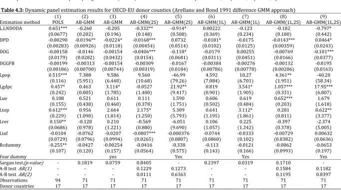
The dynamic panel GMM estimation result shows the impact of global financial crisis on ODA

disbursements. Table 4.3 and 4.4 presents the results using Arellano and Bond (1991) difference and

Blundell and Bond (1998) system GMM estimators respectively. Our analysis considered LNDODA as

a dependent variable with a lagged dependent variable and set of other explanatory variables (Eq.

3). We also present Sargan test18 _{and Arellano-Bond serial correlation test}19 _{in Table 4.3 and 4.4.}

Arellano and Bond (1991) difference GMM estimation results, considering all lags, are presented in

columns 2 of Table 4.3. The results suggest that the exogenous component of the global financial

crisis exerts a large negative impact on OECD-DAC EU ODA flows although most of the coefficients

are not statistically significant. In column 3, we considered all lags with year dummy to control for

any shocks that are common for all countries. Comparing the column 2 and 3 coefficients, the results

are not significantly different. Thus, we use 2SLS estimator considering all lags (column 4) and

coefficients are now showing more statistically significant results. Although the Sargan test supports

the validity of our estimation, the Arellano-Bond AR (2) test rejects the null hypothesis and implies

that there is second order serial correlation, which is not desirable. Next, we consider all lags with

year dummy (column 5) and employed 2SLS. The coefficients of the lagged dependent variables is

showing large negative effects (-0.914) including other variables. The negative lagged value of the

dependent variable suggests that there is no dynamic effect. Furthermore, to get more consistent

results we estimate AB-GMM considering maximum one lag (column 6) and maximum one lag with

year dummy (column 7). The coefficients values are almost identical and statistically insignificant.

18 _H

0: Instrumental variables are not correlated with error terms. he terms kjk(

, i t



, i t

[29] Table 4.2: Static panel estimation results for LDCs

(1) (2) (3) (4) (5) (6) (7) (8)

Estimation method POLS FE RE FE -AR(1) RE -AR(1) 2SLS-FE 2SLS-RE EC2SLS-RE

FDInf 0.0384 0.0400 0.0384 0.0410 0.0383 0.0661 0.0388 0.0402

(0.0512) (0.0449) (0.0512) (0.0403) (0.0519) (0.0567) (0.0543) (0.0542)

ExG -0.00614 -0.00690 -0.00614 -0.00780 -0.00576 -0.0102 -0.00610 -0.00617

(0.00721) (0.00553) (0.00721) (0.00473) (0.00730) (0.00699) (0.00807) (0.00806)

DFoR -1.52e-10 -5.40e-10* -1.52e-10 0 -1.32e-10 - - -

(4.14e-10) (3.27e-10) (4.14e-10) (2.80e-10) (4.20e-10) - - -

TEDS 4.64e-10*** 8.72e-10*** 4.64e-10*** -1.11e-10 4.33e-10*** 1.29e-09*** 3.14e-10*** 3.18e-10***

(8.97e-11) (9.69e-11) (8.97e-11) (1.15e-10) (9.03e-11) (1.09e-10) (6.31e-11) (6.29e-11)

CI 1.602** 2.267* 1.602** -0.0890 1.576** -0.236 1.409* 1.410*

(0.766) (1.213) (0.766) (1.122) (0.759) (1.502) (0.723) (0.722)

GINI 0.00323 -0.150 0.00323 -0.0842 -0.000773 -0.162 -0.0510 -0.0485

(0.0619) (0.190) (0.0619) (0.180) (0.0606) (0.240) (0.0562) (0.0562)

Pop 5.40e-08* 3.07e-07 5.40e-08* 5.84e-08 5.62e-08* - - -

(2.93e-08) (1.89e-07) (2.93e-08) (1.93e-07) (2.92e-08) - - -

NFF_Bi -3.41e-09*** -2.13e-09** -3.41e-09*** -1.27e-10 -3.41e-09*** - - -

(1.14e-09) (1.01e-09) (1.14e-09) (8.59e-10) (1.17e-09) - - -

NFF_Mu -5.40e-09*** -2.30e-09 -5.40e-09*** -2.26e-09* -5.56e-09*** -7.85e-09*** -8.17e-09*** -8.18e-09***

(1.64e-09) (1.42e-09) (1.64e-09) (1.32e-09) (1.67e-09) (1.67e-09) (1.69e-09) (1.69e-09)

MMR -1.446* -1.211 -1.446* -0.258 -1.481* 1.790* -1.050 -1.045

(0.836) (0.860) (0.836) (0.809) (0.843) (1.049) (0.847) (0.846)

AND 0.378** 0.276** 0.378** 0.220* 0.382** 0.810*** 0.490*** 0.499***

(0.155) (0.133) (0.155) (0.126) (0.156) (0.159) (0.157) (0.157)

Oda -0.00302*** -0.00355*** -0.00302*** -0.000182 -0.00299*** -0.00237*** -0.00122* -0.00154**

(0.000868) (0.000772) (0.000868) (0.000723) (0.000882) (0.000624) (0.000696) (0.000652)

XR -3.15e-05 -0.000209 -3.15e-05 -8.78e-05 -1.95e-05 -0.000192 -3.00e-05 -3.35e-05

(0.000134) (0.000339) (0.000134) (0.000340) (0.000132) (0.000427) (0.000123) (0.000123)

Wrr -1.63e-09*** -3.52e-09*** -1.63e-09*** 4.13e-10 -1.57e-09*** - - -

(2.41e-10) (3.15e-10) (2.41e-10) (4.82e-10) (2.42e-10) - - -

INF_Mor 0.0183 0.0151 0.0183 0.137** 0.0183 0.176*** 0.0198 0.0215

(0.0188) (0.0617) (0.0188) (0.0660) (0.0185) (0.0650) (0.0173) (0.0172)

Fpr 2.452*** 1.252 2.452*** 0.713 2.526*** -0.787 1.928** 1.976**

(0.875) (0.991) (0.875) (0.903) (0.878) (1.233) (0.859) (0.857)

R2 _{0.897 0.0526 0.897 0.0030 0.0939 0.0346 0.0953 0.0932}

LM test - - 56.48*** - - - - -

Baltagi-Wu test - - - 2.2512 2.2512 - - -

[30]

Table 4.2: (continued)

Observations 371 371 371 318 371 371 371 371

No. of LDCs 53 53 53 53 53 53 53 53

Note: Dependent variable is GDP per capita growth rate (RGPCG). Robust standard errors in parentheses, *** p<0.01, ** p<0.05, * p<0.1.

Table 4.3: Dynamic panel estimation results for OECD-EU donor counties (Arellano and Bond 1991 difference GMM approach)

(1) (2) (3) (4) (5) (6) (7) (8) (9)

Estimation method POLS AB-GMM AB-GMM AB-GMM(2S) AB-GMM(2S) AB-GMM(1L) AB-GMM(1L) AB-GMM(1L,2S) AB-GMM(1L,2S)

L.LNDODA 0.651*** -0.260 -0.205 -0.332** -0.914* 0.00222 -0.123 -0.182 -0.797*

(0.0677) (0.202) (0.196) (0.148) (0.508) (0.369) (0.234) (0.180) (0.442)

DPD -0.00290 -0.0196** -0.0224* -0.0168*** 0.0732 -0.0181* -0.0175 -0.0143*** 0.0464*

(0.00283) (0.00926) (0.0118) (0.00454) (0.0514) (0.0102) (0.0125) (0.00359) (0.0243)

DOG -0.00158 -0.0146 -0.00154 -0.0406*** -0.118* -0.0179 0.00255 -0.00769 -0.101***

(0.0179) (0.0282) (0.0432) (0.0154) (0.0681) (0.0311) (0.0451) (0.0166) (0.0377)

DGGFB -0.00199 -0.00313 -0.00154 -0.00309 -0.0167 -0.00384 -0.00276 -0.00132 -0.0195

(0.00186) (0.00700) (0.00744) (0.00319) (0.0184) (0.00786) (0.00778) (0.00206) (0.0163)

Lpop 0.515*** 7.388 9.586 9.560 -46.99 4.592 10.27 4.361** -40.20

(0.116) (5.951) (6.448) (10.68) (79.26) (7.084) (6.701) (1.951) (58.34)

Lgdpc 0.457* 0.463 3.114* -0.0527 21.92** 0.819 3.541* 1.057*** 17.95***

(0.242) (0.805) (1.785) (1.400) (9.417) (0.901) (1.905) (0.331) (6.807)

Lue 0.108 0.521 0.611 0.111 1.590 0.606 0.619 0.652*** 1.679

(0.155) (0.438) (0.460) (0.378) (1.751) (0.502) (0.484) (0.203) (1.618)

Ltop 0.612*** 0.956 2.664 2.175* 5.309 0.641 3.112* 0.281 8.622**

(0.229) (1.090) (1.814) (1.250) (5.793) (1.195) (1.861) (0.811) (3.377)

Lrer 0.150** -0.128 0.210 -0.569 -6.051 0.106 0.225 -0.397 -2.374

(0.0686) (0.978) (1.221) (0.880) (9.690) (1.057) (1.242) (0.378) (5.005)

Linf -0.0104 -0.0762 -0.0207 -0.0807*** -0.000376 -0.0744 -0.0333 -0.00729 0.00632

(0.0729) (0.0796) (0.0994) (0.0265) (0.0807) (0.0860) (0.102) (0.0382) (0.0636)

Bcdummy -0.255** -0.0427 -0.00254 -0.0416 -0.338 -0.113 -0.0121 -0.0862 -0.0653

(0.107) (0.120) (0.157) (0.0564) (0.575) (0.143) (0.166) (0.0993) (0.197)

Year dummy yes Yes Yes Yes

Sargan test(p-value) - 0.1819 0.0759 0.8405 - 0.2397 0.0319 0.1710 -

A-B test AR(1) - - - 0.1229 0.1273 - - 0.1584 0.1182

A-B test AR(2) - - - 0.0111 0.6363 - - 0.1195 0.8397

Observations 94 71 71 71 71 71 71 71 71

Donor countries 17 17 17 17 17 17 17 17 17

[31]

Thus, we estimate again our model using 2SLS considering maximum one lag (column 8) and

maximum one lag with year dummy (column 9). The Sargan test is not rejected, so the null

hypothesis implies the validity of our estimations and subsequently the A-B AR (2) test supports

that there is no serial correlation. However, the results of the coefficients (column 8 and 9) are still

not convincing and showing the less significant effect. The Sargan test in column 8 is not

determined as we get statistically unexpected (1.000) result, thus we estimate our model

considering Blundell and Bond (1998) system GMM estimator for our further investigation.

Table 4.4 shows the results of system GMM considering all lags, all lags with year dummy, 2-3 lags

and 2-3 lags with year dummy in column 1, 2 , 3 and 4 respectively. Except column 1, the Sargan test

statistics supports the validity of our estimations. Since the Sargan test does not reject the null

hypothesis, the instruments we used are valid. The A-B AR (2) test also suggests accepting the null

hypothesis, proposing there is no second order serial correlation of our estimations. The

coefficients of the lagged dependent variable validate the importance of including these variables.

However, the first 3 specifications (column 1-3) are showing quite similar effects. In column 1, we

found a significant effect of the lag dependent variable (0.585), but all our explanatory variables e.g.

DPD, DOG, Lpop, Lue, Ltop and Bcdummy indicate statistically insignificant results with an

estimated elasticity of -0.006, -0.05, -0.14, -0.57, -0.71 and -0.85 percent respectively. Besides, the

Sargan test reject the null hypothesis i.e. the instruments are not valid. Therefore, we carried out

further estimation considering all lags with year dummy (column 2). Since our results are quite

similar with column 1, we need to consider the further estimation. We therefore use 2SLS

estimation considering 2-3 lags with year dummy. In column 4, the test statistics supports both

validations of our instruments and there is no second order serial correlation of our model. The

coefficient of the lag dependent variable shows the lager importance with an estimated elasticity of

3.60. The positive lagged value of the dependent variable suggests the existence of significant

[32]

Table 4.4: panel estimation results for OECD-EU donor counties (Blundell and Bond 1998 system GMM approach)

(1) (2) (3) (4)

Estimation method System GMM System GMM System GMM (2-3L) System GMM (2-3L)

L.LNDODA 0.585** 0.270 0.339 3.600**

(0.270) (2.064) (0.227) (1.727)

DPD -0.00617 0.290* -0.0151 0.209*

(0.00807) (0.172) (0.0150) (0.118)

DOG -0.0538 -1.116 -0.0391 -0.518

(0.0578) (1.132) (0.0298) (0.468)

DGGFB 0.0225 -0.0866 0.0261 -0.162**

(0.0328) (0.128) (0.0180) (0.0788)

Lpop -0.141 1.787 0.174 -1.235

(1.224) (4.198) (0.373) (1.818)

Lgdpc 2.372 30.34 2.762* -0.114

(2.502) (29.41) (1.464) (4.251)

Lue -0.560 -0.389 0.119 -3.418

(1.405) (1.717) (0.752) (4.967)

Ltop -0.715 8.173 -0.518 6.782*

(2.769) (12.55) (0.906) (3.549)

Lrer 1.006 -12.51 1.730 -16.50*

(0.730) (12.95) (1.162) (9.124)

Linf 0.0678 -2.837 -0.0423 1.332

(0.176) (1.828) (0.118) (4.658)

Bcdummy -0.854 -1.886 -0.689** -5.276**

(0.975) (3.560) (0.296) (2.191)

Year dummy yes Yes

Sargan test(p-value) 0.046 0.121 0.115 0.942

A-B test AR(1) 0.016 0.214 0.012 0.280

A-B test AR(2) 0.406 0.913 0.715 0.712

Observations 94 94 94 94

Donor countries 17 17 17 17

Note: Dependent variable is log of net ODA (LNODA). Robust standard errors in parentheses, *** p<0.01, ** p<0.05, * p<0.1. (1) System GMM, Blundell and Bond (1998) system GMM considering all lags; (2) System GMM, Blundell and Bond (1998) system GMM considering all lags with year dummy; (3) System GMM (2-3L), Blundell and Bond (1998) system GMM considering max 2-3 lags; (4) System GMM (2-3L), Blundell and Bond (1998) system GMM considering max. 2-3 lags with year dummy;

This result also explores that general government fiscal balance (DGGFB), real exchange rate (Lrer)

and banking crisis dummy shows significant negative effect on ODA flows. Subsequently, output gap

(DOG), and unemployment rate (Lue) also depict considerably negative effects although its not

statistically significant.

In short, the finding of the OECD-DAC EU donor countries dynamic panel analysis (Eq. 3) revealed

that global financial crisis affects ODA flows to the LDCs. This is also supported by our static panel

data analysis (Eq. 1). Our estimation results indicate that OECD-DAC EU donors tended to provide