Algorithm for construction of portfolio of stocks using Treynor’s ratio

Algorithm for construction of portfolio of

stocks using Treynor’s ratio

Sinha, Pankaj and Goyal, Lavleen

Faculty of Management Studies, University of Delhi

7 July 2012

Online at

https://mpra.ub.uni-muenchen.de/40134/

Page 1

Algorithm for construction of portfolio of stocks using

Treynor’s ratio

Pankaj Sinha

Faculty of Management Studies, University of Delhi Lavleen Goyal

Indian Institute of Technology, Guwahati

Abstract

Page 2

1. Introduction

Market offers several assets in various formats which are grounds for investing money and gaining returns after specific time periods. Investments are made in view of obtaining highest returns with lowest chance of losing money. The returns are however characterised by the nature of assets and the market factors that influence its pricing everyday. Since the returns cannot be foretold with certainty, the analysis of profitability in an asset becomes an objective of utmost priority in an investment procedure. A technique of judging the behaviour returns from an asset is historical data analysis of the asset with respect to market.

The classic portfolio theory of Markowitz[1] shows that a collective group of assets if formulated using mathematical modelled optimisation problem, can give higher returns with lower chance of losing money. In fact, Markowitz portfolio model gives the most basic and complete framework for investment decision. On the negative end, Markowitz theory exhausts the chances of selecting the asset that give unusual higher return on the cost of volatility.

This paper uses Treynor’s ratio (i.e. excess return to beta) as the criteria for the selection of a stock in a portfolio as described in Elton, Gruber, Brown and Goetzmann[2]. The algorithm gives the percentage weights to be invested in each stock selected without short selling, for an optimum portfolio by evaluating the historical data available on stocks.

2. The decision making procedure of Treynor’s ratio

Suppose we are having a pool of stocks of an index and we want to select stocks and calculate the weights of the selected stocks to be invested. The desirability of a stock is directly proportional to “excess return to beta” ratio i.e. Treynor’s ratio. Excess return is the difference between the rate of return of the stock and the risk free rate of return as on Treasury bill (say). Beta specifies the non diversifiable risk (risk which cannot be eliminated by diversification).

Treynor’s ratio= (E[Ri] – Rf )/βi

where βi =beta value of the stock (the relative change in excess return of stock with 1% change in market)

E[Ri] = Expected return of ith stock Rf = risk free rate

Page 3

the stocks with the higher treynor’s ratio than this C* are selected for portfolio construction. The procedure of finding C*, as given in Elton, Gruber, Brown and Goetzmann[2], involves finding Ci for each stock assuming ith stock is present in our optimum portfolio.

Ci = σm2 ∑ [{(E[Rj]-Rf) βj}/σej2] 1 + σm2∑ ( βj2/σej2) where σm = market volatility

σej2 = unsystematic risk of stock (risk not related to market but stock’s nature) βj = beta value of the stock (index of systematic risk present in the jth stock) E[Rj] = Expected return of jth stock

Rf = risk free rate

Out of these Ci’s, there will be only one Ci for which treynor’s ratio of all the stock preceding this ith stock will be greater than this Ci and treynor’s ratio of all the succeeding this ith stock will be less than this Ci. This Ci will be our C* and all the stocks preceding it will be selected in our optimum portfolio.

3. Calculation of weights of stock in our optimum portfolio

The weightage of capital invested in each selected stock (Xi) can be calculated as given in Elton, Gruber, Brown and Goetzmann[2].

Xi = Zi ∑ Zi

where Zi = (βi/σei2) [{(E[Ri]-Rf)/ βi} - C*]

4. Algorithm

The algorithm requires an input of adjusted closing price of pool of stocks and of the market index. Following are the steps involved in our algorithm. The complete MATLAB program is given in the Appendix.

§ The data is read from the excel files and daily return of all the stocks as well as market is calculated as

r(i) = V(i+1)-V(i) . V(i)

§ Average daily return is calculated by using the geometric mean of the historical daily returns as given by

DR=((1+r1)(1+r2)(1+r3)(1+r4)…(1+rn))1/n -1

Page 4

§ Average annual return is calculated from average daily returns assuming 252 trading days in a year.

AR = (1+DR)252-1

Annual standard deviations can be calculated from the daily standard deviations as

Astd = √252× Dstd

§ Capital Asset Pricing Model is used to calculate the raw beta for each stock which states the dependence of expected return of an asset on the market movement.

Ri(t) = Rf + βi {Rm(t)-Rf} + εi where Ri –Rf = excess return of asset

Rm- Rf = excess return of market εi = shock factor with mean =0

Linear regression is run for each stock on excess daily return of stock vs. excess daily return of market for finding the raw beta as per historical data. Then the adjusted beta(Aβ) is calculated from the raw beta(Rβ) assuming that the security’s beta move towards the market average over time with a 67% confidence level as given by

Aβ = 0.67*Rβ + 0.33*1

§ The stocks with β coming out to be –ve are removed.

§ Now the investment decision is made on the basis of Treynor’s ratio as described above and the weights of the accepted stocks are calculated.

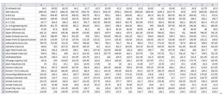
5. Application Example

We have considered index of S&P CNX 500 and the underlying stocks in the index for implementing the above algorithm using MATLAB, for the period June-2010 to June-2012.

Inputs :

Page 5 …

Figure 1 : Adjusted closing price of stock

§ The closing price of the market index is taken from NSE website and kept in the file “market.xlsx” as shown in the figure 2.

…

Figure 2 : Closing price of market index (S&P CNX 500)

§ Risk free rate is taken as per rate of treasury bills given on RBI website.

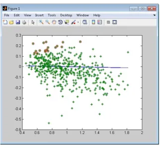
Output of the above algorithm:

Page 6

Figure 3 : Security Market Line(Blue Line)

Green points show the positions of stock and the selected stocks are circled with red colour

Figure 4 : The list of stocks selected for optimum portfolio with their corresponding weights

The performance of the portfolio constructed from the above selected 17 stocks is given in the table 1.

Page 7

Sharpe ratio 3.60 Jensen’s alpha 65.28%

Table 1 : Performance of the obtained portfolio

6. Conclusion

We found that our optimum portfolio gives an annual return of 67.22% with respect to risk free return of 7.966%. This shows that the given method is very effective in investment decision making and even in today’s economic scenario and investment environment in India, we can still achieve such good returns by selecting stocks using the described methodology and algorithm.

7. References

[1] H.M. Markowitz, “Portfolio Selection”, Journal of Finance,7(1952),77-91 [2] E.J. Elton, M.J. Gruber, S.J. Brown, W.N. Goetzmann, Modern Portfolio Theory and Investment Analysis, (2009)

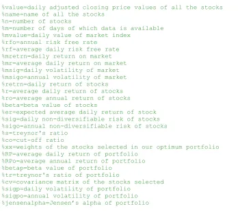
8. Appendix

%DEFINITION AND NAMES OF VARIABLES USED

%value=daily adjusted closing price values of all the stocks %name=name of all the stocks

%n=number of stocks

%m=number of days of which data is available %mvalue=daily value of market index

%rfo=annual risk free rate %rf=average daily risk free rate %mretrn=daily return on market %mr=average daily return on market %msig=daily volatility of market %msigo=annual volatility of market %retrn=daily return of stocks %r=average daily return of stocks %ro=average annual return of stocks %beta=beta value of stocks

%er=expected average daily return of stock %sig=daily non-diversifiable risk of stocks %sigo=annual non-diversifiable risk of stocks %s=treynor's ratio

%co=cut-off ratio

%xx=weights of the stocks selected in our optimum portfolio %RP=average daily return of portfolio

%RPo=average annual return of portfolio %betap=beta value of portfolio

%tr=treynor's ratio of portfolio

%cv=covariance matrix of the stocks selected %sigp=daily volatility of portfolio

Page 8

%MAIN PROGRAM

close all; clear all;

[value,name]=xlsread('DATA.xlsx'); [n,m]=size(value);

[mvalue]=xlsread('market.xlsx'); rfo=7.966;

rf=100*(((1+rfo/100)^(1/m))-1);

for i=1:(m-1)

mretrn(i)=100*(mvalue(i+1)-mvalue(i))/mvalue(i);

end

mr=100*(geomean(1+mretrn/100)-1); msig=std(mretrn);

msigo=sqrt(252)*msig;

for i=1:(m-1)

retrn(:,i)=100*(value(:,i+1)-value(:,i))./value(:,i);

end

for i=1:n

r(i)=100*(geomean(1+retrn(i,:)/100)-1); ro(i)=100*(((1+(r(i)/100))^252)-1);

end

for i=1:n

y=retrn(i,:)'-rf; x=(mretrn-rf)'; temp1=ones(m-1,1); x=[temp1 x]; temp2=inv(x'*x)*x'*y; beta(i)=temp2(2); beta(i)=0.67*beta(i)+0.33; end flagg=0; while(flagg==0)

for i=1:n

if(beta(i)<0 || beta(i)==NaN) beta(i)=[]; value(i,:)=[]; retrn(i,:)=[]; r(i)=[]; ro(i)=[]; n=n-1; break; flagg=0; else flagg=1; end end end er=rf+beta*(mr-rf); plot(beta,er) hold on;

for i=1:n

sig(i)=sqrt((std(retrn(i,:)-rf)^2)-(beta(i)^2)*(std(mretrn-rf)^2)); sigo(i)=sqrt(252)*sig(i);

s(i)=(ro(i)-rfo)/beta(i);

end

[s,order]=sort(s,'descend'); beta=beta(order);

Page 9 r=r(order); ro=ro(order); retrn=retrn(order,:); sum1=0; sum2=0; flag=0;

for i=1:n

sum1=sum1+((ro(i)-rfo)*beta(i))/(sigo(i)^2/100); sum2=sum2+(beta(i)^2)/(sigo(i)^2/100); c(i)=((msigo^2/100)*(sum1))/(1+(msigo^2/100)*(sum2)); if(c(i)<s(1:i)) if(c(i)>s((i+1):n)) co=c(i); io=i; flag=1; end end end

scatter(beta,r,'*') hold on;

if(flag==1)

for i=1:io

z(i)=(beta(i)/(sig(i)^2/100))*(((ro(i)-rfo)/beta(i))-co);

end

for i=1:io

xx(i)=z(i)/sum(z);

end

xlswrite('output.xlsx',name(1:io),'A1:A10000'); xlswrite('output.xlsx',xx(1:io)','B1:B10000'); scatter(beta(1:io),r(1:io),'red')

RP=sum(xx(1:io).*r(1:io)); RPo=100*(((1+RP/100)^252)-1) betap=sum(xx(1:io).*beta(1:io)) tr=((RPo-rfo)/betap) cv=cov(retrn(1:io,:)'); sigp=sqrt(xx*cv*xx'); sigpo=sqrt(252)*sigp sr=(RPo-rfo)/sigpo temp=RP-(rf+betap*(mr-rf)); jensenalpha=100*(((1+temp/100)^252)-1) else