Munich Personal RePEc Archive
On the Continuous Equilibria of
Affiliated-Value, All-Pay Auctions with
Private Budget Constraints
Kotowski, Maciej and Li, Fei
Harvard Kennedy School, University of Pennsylvania
20 March 2011
On the Continuous Equilibria of Affiliated-Value,
All-Pay Auctions with Private Budget Constraints
Maciej H. Kotowski
∗Fei Li
†January 4, 2012
Abstract
We consider all-pay auctions in the presence of interdependent, affiliated valuations and private budget constraints. For the sealed-bid, all-pay auction we characterize a symmetric equilibrium in continuous strategies for the case of N bidders and we in-vestigate its properties. Budget constraints encourage more aggressive bidding among participants with large endowments and intermediate valuations. We extend our re-sults to the war of attrition where we show that budget constraints lead to a uniform amplification of equilibrium bids. An example shows that with both interdependent valuations and private budget constraints, a revenue ranking between the two mecha-nisms is generally not possible.
JEL: D44
Keywords: All-Pay Auction, War of Attrition, Budget Constraints, Common Values, Private Values, Affiliation, Contests
∗Harvard Kennedy School, Cambridge MA 02138. E-mail: maciej [email protected]
Suppose firms are lobbying for a lucrative government contract. Clearly, the contract’s value to each firm has an idiosyncratic component since the firms likely have different op-erating costs. On the other hand, each firm also has a privately known limit on how much it is able or willing to spend on the lobbying game. Perhaps the management of one firm is approving of small restaurant meals with officials but expenditures or bribes beyond some threshold are morally too much to stomach. A competitor, in contrast, may be less ham-pered in its lobbying strategy. How does the lobbying game unfold when competitors differ in their valuation for the prize and in their ability or capacity to compete for it? Would some firms spendmore on lobbying believing that their competitors have to navigate within some private constraints on actions?
In this essay we consider the class of situations like the above by analyzing the all-pay auction. In an all-pay auction, the highest bidder is the winner of the item for sale; however, all bidders incur a payment equal to their bid. As a stylized model of a lobbying contest, the all-pay auction has a long tradition in political economy (Baye et al., 1993).
Despite the frequent application of the all-pay auction to contests, most analyses fail to capture the exogenous but private limits on actions that are relevant in many situations. We introduce these constraints into the all-pay auction and we identify sufficient (and from a practical perspective necessary) conditions for the existence of an equilibrium in continuous strategies. Our analysis isolates a general amplification of bids submitted by bidders with intermediate valuations. An extension of our model to the war of attrition shows the general-ity of the bid amplification phenomenon and allows for a comparison of the revenue potential of the two mechanisms. Generally, no revenue ranking exists between the two formats in the presence of both budget constraints and affiliated, interdependent values.
naturally modeled as either an all-pay auction or as a war of attrition (Leininger, 1991). The expected value of the invention and the budget available to the research division will deter-mine the effort devoted to the race. However, information asymmetries or agency concerns can create a wedge between the available budget and the research division’s assessment of the project’s value. Moreover, a firm as a whole likely faces a hard, short-run resource con-straint that will cap its feasible effort level. It is natural to suppose that this resource limit is also private information. The interaction between expected rewards and the heterogenous resource constraints will shape how firms engage in this competition.
While we are motivated by the range of applications of all-pay auctions in modeling social and economic situations, our study also fills a gap in the small but growing literature on auctions with private budget constraints. Our analysis begins with the work of Krishna & Morgan (1997) who study the all-pay auction and the war of attrition with interdependent and affiliated valuations. To this setting we introduce private budget constraints distributed continuously on an interval. Our environment parallels the setting of Fang & Parreiras (2002) and Kotowski (2010) who study the second-price and the first-price auction with private budget constraints respectively. Both of these studies build on Che & Gale (1998), which is the seminal paper in this strand of literature.
In light of this literature, our study contributes along several dimensions. First, by focusing on all-pay mechanisms we put under scrutiny an important allocation mecha-nism in resource-constrained environments. Many authors examining optimal auctions with budget-constrained participants have resorted to mechanisms that feature “all-pay” pay-ment schemes (Maskin, 2000; Pai & Vohra, 2011). Our analysis therefore complepay-ments this literature but we do not attempt the mechanism design exercise here.
Second, by developing our model in a more general setting than traditionally employed we are able to identify additional features of the environment that affect the existence of a well-behaved and (relatively) tractable equilibrium. Previous studies lodged in the affiliated and interdependent-value paradigm, such as Fang & Parreiras (2002) and Kotowski (2010), have focused exclusively on the bidder case. While some of the intuition from the two-bidder case is relevant generally, the case of two two-bidders masks much of the nuance that we identify. For example, in the all-pay auction we document how changes in the number of bidders alone directly affects the existence of an equilibrium within the class of strategies traditionally considered by this literature.
In particular, we endeavor to employ more localized assumptions whenever possible. For example, we do not require differentiability or continuity conditions on the distribution of budgets over its entire range. Similarly, we do not need the existence of an unambiguously unconstrained bidder.1 Accommodating weaker assumptions renders our argument more
involved than previous analyses in this environment.
Although we relax many assumptions, we do not study the all-pay auction’s equilibrium in its fullest generality. Indeed, from the onset we focus on the existence of an equilibrium that is continuous, symmetric, and monotone. We view this restricted scope to be a pragmatic but reasonable choice. From a technical perspective, this restriction allows us to define equilibrium behavior as a solution to a differential equation. This methodology offers a window on the mechanism’s economic properties and gives precise predictions concerning bidder behavior. We believe that the set of cases covered is rich and it offers insights that would carry over to any discontinuous (but symmetric and monotone) equilibrium. Moreover, continuous equilibria would receive the bulk of attention in applications due to their relative tractability.
The remainder of the paper is organized as follows. Section 1 introduces the model and section 2 characterizes our symmetric equilibrium in the all-pay auction. We then consider the equilibrium’s comparative static properties with focus on changes in the distribution of budgets, changes in the number of bidders, and changes in the public information surround-ing the contest. The final section considers this model’s second-price analogue, the war of attrition. We explore the symmetric equilibria of this model and we discuss the scope for a revenue ranking. Proofs and supporting lemmas are in the appendix.
1
The Environment
Let N ={1, . . . , N} be the set of bidders. Each bidder i ∈ N observes a two-dimensional private signal (si, wi)∈Θ⊂R2+. We allow for both Θ = [0,1]×[w,w¯] and Θ = [0,1]×[w,∞)
but for brevity we will phrase our model in the former case. A bidder’s realized value-signal,
si, is her private information about the item for purchase. For example, in a patent race it
would be an estimate of the invention’s value. Let s = (s1, . . . , sN) be a profile of realized
value-signals.2 We use capital letters—Si, etc.—to refer to signals as random variables.
A bidder’s realized budget, wi, is a limit above which she cannot bid. We consider a
1There exists an unambiguously unconstrained bidder if with positive probability there exists a participant
with a budget in excess of the maximum possible value of the item.
2We use standard notation: s
budget to be a hard constraint on expenditures. A budget may correspond to a bidder’s cash holdings, her credit limit, or some other private limit on actions. Alternatively, budget constraints can be modeled as “soft” constraints acting through an increasing cost of bidding. For brevity, we do not explore this extension. Zheng (2001), among others, is an application of this specification of budget constraints.
We assume that bidder i’s valuation for the item can be described by a random variable:
Vi =u(Si, S−i). We assume that u: [0,1]×[0,1]N−1 →[0,1] is strictly increasing in the first
argument and nondecreasing and permutation-symmetric in the last N −1 arguments. As standard, we suppose uis continuously differentiable and normalized such thatu(0, . . . ,0) = 0 and u(1, . . . ,1) = 1.
A bidding strategy is a (measurable) functionβi: Θ →R+. LetS be the set of strategies.
A strategy is nondecreasing if s′
i ≥ si and w′i ≥wi imply βi(s′i, w′i)≥ βi(si, wi). A strategy
is strictly increasing if it is nondecreasing and βi(s′
i, wi′) > βi(si, wi) when either s′i > si
or w′
i > wi. Throughout, we adopt Bayesian Nash equilibrium as our solution concept.
An equilibrium is symmetric if all bidders follow the same bidding strategy. We focus on symmetric equilibria and we henceforth suppress player subscripts in our notation whenever possible.
We always assume that bidders are risk neutral. The introduction of risk aversion into this model introduces complications analogous to those seen in the first-price auction. As shown by Kotowski (2010), the interaction of a bidder’s private budget with her risk preferences can introduces countervailing incentives rendering the existence of “monotone” equilibria a more involved question.
We begin with two assumptions on the ambient environment which we maintain through-out. Our initial set-up is standard. Subsequently, we will impose additional restrictions on the information structure that will be sufficient for equilibrium existence. The additional conditions will be specific to the auction format; therefore, we introduce them separately.
Assumption 1. The distribution of value-signals satisfies the following conditions:
(a) Value-signals have a joint densityh(s1,· · · , sN)which is continuous and strictly positive:
0< h(s1,· · · , sN) for all (s1,· · · , sN)∈[0,1]N.
(b) h(s1,· · · , sN) is invariant to permutations of (s1, . . . , sN).
Affiliated signals are a standard assumption introduced to the auction literature by Milgrom & Weber (1982).3 Except for budget constraints, our model corresponds to their classic
environment. Affiliation allows some correlation in player’s information. Although more general than independence, it is nonetheless a strong assumption (de Castro, 2010).
Our second assumption about the ambient environment concerns the distribution of a player’s budget.
Assumption 2. Players’ budgets are independently and identically distributed according to the cumulative distribution function G: [0,∞)→[0,1]. If w(w¯) is the infimum (supremum) of the support ofG, thenG(w) = 0. Moreover, budgets are distributed independently of value-signals.
While the independence assumption is strong, without it the model is not tractable. It is standard in studies of auctions with budget constraints. We emphasize that w need not be zero and ¯w need not be infinite. Indeed, in many situations it would be unreasonable to suppose this to be the case. For example the parameters of the support of G may become common knowledge via posted bonds, (not modeled) participant selection, or obligatory financial disclosures as may occur in the context of political lobbying. In future work we intend to explore the effects of endogenous disclosure ofw (or ¯w) but for now we take them as given and common knowledge.
2
A Symmetric, Continuous Equilibrium in the
All-Pay Auction
The rules of the all-pay auction are well-known. Each bidderi will simultaneously submit a bid bi. A bid must be feasible given the bidder’s budget: bi ≤ wi. If bidder i submits the highest bid she wins the game and her payoff under the realized signal profile s = (si,s−i)
is u(si,s−i)−bi; otherwise, it is −bi. Ties among high bidders are resolved by a uniform
randomization to designate the winner.
We endeavor to identify a symmetric equilibrium where all bidders follow a strategy of the form
β(s, w) = min{b(s), w} (1) where b: [0,1] → R+ is strictly increasing, continuous, and piecewise differentiable. Let
M ⊂ S denote the set of strategies that meet these criteria. We will say that an auction has
an equilibrium inMif there existsβ ∈ M which is a symmetric Bayesian Nash equilibrium. Our focus on equilibria meeting these criteria is consistent with previous studies of auctions with private budget constraints. Che & Gale (1998), Fang & Parreiras (2002, 2003), and Kotowski (2010) examine equilibria that reside in this class of strategies.
To motivate the sufficient conditions for equilibrium existence that we propose below, we begin with an heuristic discussion. Suppose for the moment that there is a symmetric equilibrium β(s, w) = min{b(s), w} ∈ M and consider a bidder of type (s, w). If this player bids b(x)≤wher bid will defeat two categories of opponents assuming all other bidders are following the strategyβ(s, w). First it defeats all opponents who have a value-signals < x. Second, it defeats all opponents who have a budget w < b(x) irrespective of value-signal. Since β(s, w) is strictly increasing, ties are probability zero events.
To succinctly express a bidder’s expected payoff from the bid b(x) require new notation, which we use recurrently. First, for each k let
zk(x|s)≡
Z 1
0
· · ·
Z 1
0 | {z }
N−1−k
Z x
0
· · ·
Z x
0 | {z }
k
u(s, y1, . . . , yN−1)h(y1, . . . , yN−1|s)dy1· · ·dyN−1. (2)
In (2) we have omitted the subscript for player i and we have relabeled theN−1 signals of the other bidders as (y1, y2, . . . , yN−1).4 Second, for each k define
Fk(x|s) =
Z 1
0 · · · Z 1
0 | {z }
N−1−k
Z x
0 · · · Z x
0 | {z }
k
h(y1, . . . , yN−1|s)dy1· · ·dyN−1. (3)
For k ≥ 1, Fk(x|s) is the cumulative distribution function of the random variable ¯Yk = max(Y1, . . . , Yk) givenS =s. Letfk(x|s) be the associated density function. Third, if we let
vk(s, y)≡E[u(s, Y1, . . . , YN−1)|S =s,Yk¯ =y],
then by Lemma 17 we can write
zk(x|s) =
Z x
0
vk(s, y)fk(y|s)dy. (4)
Depending on the circumstances we may express zk(x|s) in form (2) or (4).5 4We do not reorder the signals of the other bidders from greatest to least.
5We adopt the following conventions: z0(x
Defining
γk(b)≡
N−1
k
G(b)N−1−k(1−G(b))k, (5) we can write the bidder’s expected payoff from the bidb(x) as
U(b(x)|s, w) =
N−1 X
k=0
γk(b(x))zk(x|s)−b(x). (6)
The binomial terms account for the combinations of opponents who are defeated byb(x) due to having a low value-signal or a low budget. We do not need to keep track of the precise identities of these bidders due to the symmetry assumptions on both valuations and informa-tion structure. Introducing asymmetries would necessitate a more detailed accounting of the different cases. The final term in (6) is the bidder’s payment which she makes irrespective of the auction’s outcome.
Ifb(s)< wis indeed this player’s equilibrium best response, a local first-order optimality condition must be satisfied. Specifically, if U(b(x)|s, w) is sufficiently smooth then
d
dxU(b(x)|s, w)
x=s
= 0. (7)
Adopting the notation
zk′(x|s)≡ ∂
∂xzk(x|s) =
0 if k = 0
vk(s|x)fk(x|s) ifk 6= 0 (8) we can evaluate (7) to derive the following differential equation:
b′(s) =
PN−1
k=0 γk(b(s))z′k(s|s)
1−PNk=0−1γk′(b(s))zk(s|s)
. (9)
Our subsequent discussion will identify conditions that ensure (9) has a sensible solution which we later confirm is characteristic of equilibrium bidding.
Two initial observations are worthwhile. First, when b(s)< w equation (9) reduces to
b′(s) =vN−1(s, s)fN−1(s|s)
which is the differential equation identified by Krishna & Morgan (1997) as characterizing bidding behavior in the all-pay auction absent budget constraints. Therefore, our sufficient conditions must suitably generalize their assumptions. Second, when b(s)> w, (9) accounts for the change in marginal incentives faced by unconstrained bidders. Slight bid increases not only defeat opponents with slightly higher valuations but they also defeat all opponents with sufficiently low budgets regardless of their valuation. This second effect ameliorates the well-known winner’s curse phenomenon in interdependent-value settings.
Regrettably the derivation of (9) was heuristic and we made many implicit assumptions. First, to render the differential approach valid, we will need to impose some degree of smooth-ness on the distribution of budgets,G(w), and we will need to ensure that the solution of (9) is contained in a region where G(w) is smooth. Second, even if (9) can be solved, it is not clear that anincreasing solution on all of [0,1] exists. For example, if the denominator of (9) is ever negative, then b′(s)<0 contradicting our original hypothesis that b(s) is increasing.
Finally, we must also be mindful of boundary conditions, which we have not yet considered. To address the above points and to identify sufficient conditions when (9) does charac-terize equilibrium bidding we introduce three additional assumptions. Our first assumption will makeG(w) continuously differentiable in a relevant range of values. The second assump-tion will limit the degree of affiliaassump-tion among bidder’s value-signals. The final assumpassump-tion will place a restriction on the joint distribution of value-signals and budgets. While the first assumption is strictly technical, the latter two assumptions speak to the complicated interaction among incentives faced by bidders in the all-pay auction. We elaborate on these assumptions below.
We begin our analysis by introducing the function
α(s)≡
Z s
0
vN−1(y, y)fN−1(y|y)dy. (10)
Krishna & Morgan (1997) show that under suitable conditions α(s) defines the equilibrium bidding strategy in the all-pay auction without private budget constraints. Let ¯α = α(1). This value will emerge as an upper bound on equilibrium bids in our model and with reference to it, we can present our first restriction.
Assumption 3. G(·) is continuously differentiable on [w,α¯] and its derivativeg(w) on this interval is strictly positive. Moreover, w <α <¯ w¯.
G(w) to be differentiable for all w≤1. However, on terms relative the equilibrium and the auction format, we consider it to be of an equivalent character to their assumption.
The next assumption generalizes the sufficient condition proposed by Krishna & Morgan (1997) supporting α(s) as the equilibrium strategy in the all-pay auction without budget constraints.
Assumption 4. For all s−i ∈[0,1]N−1, u(·,s−i)h(s−i|·)→R+ is nondecreasing and
differ-entiable.
Intuitively, Assumption 4 limits the degree of correlation between value-signals relative to the impact of a player’s own signal on her valuation. The assumption always holds if signals are independent but it can hold in other cases as well. For example it is satisfied when there are two bidders, u(si, sj) = (si+sj)/2 and h(si, sj)∝1 +sisj.
Whereas Assumption 4 places a restriction on the correlation among only value-signals, we additionally require an assumption structuring the joint distribution of value-signals and budgets. Assumption 5 presents this restriction. We defer interpreting this assumption until after presenting our main result and an example illustrating the identified equilibrium.
Definition 1. The value ˜s∈[0,1) is the unique solution to α(˜s) = w.
Assumption 5. For all (x, s)∈[0,1]2 and for all w∈[w,α¯], define
ξ(x, w|s) =γ0(w) +
N−1 X
k=1
γk(w)
1− kg(w)
1−G(w)(zk−1(x|s)−zk(x|s))
. (11)
Then the following conditions hold:
(a) For alls≥s˜, ∃ws ∈[w,α¯)such thatw∈[w, ws) =⇒ ξ(s, w|s)<0andw∈(ws,α¯] =⇒
ξ(s, w|s)>0.
(b) If s >˜ 0, there exists ǫ >0 such that for all s ∈(˜s−ǫ,s˜+ǫ), ξ(s, w|s)>0.
Proposition 1. Suppose Assumptions 1–5 are satisfied. Then there exists a continuous, symmetric equilibrium of the all-pay auction with budget constraints of the form β(s, w) = min{b(s), w}whereb(s)is a continuous, strictly increasing, and piecewise differentiable func-tion such that
b(˜s) = inf{w > w:ξ(˜s, w|s˜)>0}, (12)
and for almost every s, b′(s) = PNk=0−1γk(b(s))z′k(s|s)
1−PN−1 k=0 γ
′
Remark 1. When w >0, condition (12) reduces tob(˜s) =w.
The following example highlights several features of the equilibrium of the all-pay auction.
Example 1. SupposeN = 2 and that value-signals are given bySi i.i.d.∼ U[0,1] while budgets
Wi i.i.d.∼ U[2 25,
3
4]. Let u(si, sj) = (si+sj)/2.
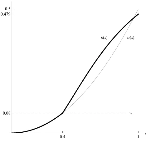
It is readily verified that b(s) =s2/2 for s < ˜s = 2
5. Of course, α(s) = s
2/2 is also the
equilibrium strategy in this model absent budget constraints. For s > 25,b(s) is the solution to the differential equation
b′(s) = 25(3−4b(s))s 25s(3s−2) + 42
satisfying the boundary condition b 25= 252. The resulting equilibrium strategy is
β(s, w) =
s2
2 s≤
2 5
min{b(s), w} s > 25
[Figure 1 about here.]
Figure 1 plots the functions b(s) andα(s) = s22.6 The introduction of budget constraints
rendered b(s) concave for s > s˜ while α(s) is convex. This pronounced change is not a general phenomenon; in other examples b(s) remains convex throughout. What is a general phenomenon, however, is the more aggressive bidding of some types of bidders. To the right of ˜s = 25, b(s) > α(s). Additionally, bidders with very high valuations s → 1 bid less aggressively than in the corresponding equilibrium in this environment without budget constraints. These equilibrium characteristics apply generally as shown by the following corollaries.
Corollary 1. Suppose the conditions of Proposition 1 hold and w >0. (a) lims→s˜+b′(s)>lims→s˜−b′(s) = lims→s˜−α(s).
(b) For all (s, w), β(s, w)≤α(1).
The encouragement of more aggressive bidding by bidders with relatively large budgets and intermediate valuations is due to the change in marginal incentives that bidders experi-ence in the presexperi-ence of budget constraints. The prospect of defeating additional opponents who are budget constrained increases the marginal return of a higher bid; therefore, some types of bidders respond to this incentive with more aggressive bidding.
Discussion and Interpretation
To interpret the sufficient conditions behind Proposition 1 it is useful to examine in detail the role of Assumption 5. Assumption 5(a) asserts that the functionξ(s,·|s) satisfies a single crossing condition and is strictly positive forwsufficiently close to ¯α.7 As shown by Lemma
14, ξ(x, w|s) = 1−PkN=0−1γk′(w)zk(x|s). Thus, the assumption ensures that the righthand
side of the differential equation (9) is eventually strictly positive. While this is Assumption 5’s technical role, it also has an economic interpretation that we outline below.
With Lemma 14, we can write the condition ξ(s, w|s)>0 as
g(w)(N −1)
"N−2 X
k=0
N −2
k
G(w)N−2−k(1−G(w))k(zk(s|s)−zk+1(s|s)) #
<1.
To simplify further suppose values are private and value-signals are independent draws from a common distribution with c.d.f. H(s). In this case:
zk(s|s)−zk+1(s|s) = u(s)H(s)k(1−H(s)).
ξ(s, w|s)>0 now becomes
g(w)(N −1)u(s)(1−H(s)) (G(w) +H(s)−G(w)H(s))N−2 <1
⇐⇒ u(s) d
dw[G(w) +H(s)−G(w)H(s)] N−1
<1.
The term [G(w) +H(s)−G(w)H(s)]N−1 is the probability of all other bidders having a signal less than s and/or a budget less than w. If b = β(s, w) as equilibrium bidding assumes, this would be the probability with which bidder i wins the auction with a bid of
b. We can therefore regard Assumption 5 as imposing a limit on the rate of change in the probability of winning owing only to defeating opponents who have a smaller budget. If this probability increases too rapidly at some point ˆw—for instance, due to an “atom”8 in the
distribution of budgets—then asb(s) crosses ˆw,b′(s) becomes undefined or negative and the
continuous strategy we are considering can no longer be an equilibrium.
In an interdependent-value setting, the preceding intuition continues to apply. However,
7ξ(s,
·|s) may become negative forw >α¯.
8We are assuming atomless distributions of budgets, but the intuition in the case of an atom offered
here is illuminating. In the atomless framework, suppose that g( ˆw) > N −1 while g(w) < 1
it must be extended to incorporate the winner’s curse. Defeating low-budget opponents is generally “good news” concerning the expected value of the item. Therefore in its fullest form, (11) additionally incorporates a weighted average controlling for these marginal effects on an opponent-by-opponent basis.
Since the sufficient conditions in Assumption 5 may be difficult to verify in practice, a simple (but exceptionally conservative) alternative is given by the following lemma.
Lemma 1. Assumption 5 is satisfied if g(w)(N −1)E[u(1, Y1, . . . , YN−1)|S = 1]< 1 for all
w∈[w,α¯].
Effectively, this lemma places a uniform limit on the preponderance of budget constraints in the relevant range of bids. Of course, this strict limit is not necessary for equilibrium existence. Example 1 presented above does not satisfy the condition of Lemma 1.
The proof of Proposition 1 is presented in the Appendix and it follows several steps. First, we consider the situation where g(w) exists and is continuous for all [w,w¯]. In ad-dition, it satisfies a specific bound when w > α¯. This bound is defined in a self-referential manner; therefore, we verify that there exist distributions that indeed meet it and fulfill our other assumptions. The bound ensures that the single-crossing assumption imposed on ξ
is sufficient to ensure that relevant solutions to (9) are increasing. We then argue that an appropriate solution to (9) is defined for all [˜s,1] when the distribution of budgets satisfies our bound. Finally we show that the solution, b(s), is bounded above by ¯α. To confirm this fact requires a definition forb(s) for all [˜s,1] and for b(s) to be strictly increasing; therefore, our sequencing of the argument is important.
We conclude by considering the wider class of distribution functions allowed by Propo-sition 1. We show how any G meeting the maintained assumptions can be transformed to a distribution meeting the aforementioned bound while preserving its values for w ≤ α¯. The solution for b(s) in the transformed situation will be a solution in the original en-vironment. Having established that b(s) exists and that it satisfies (9), confirming that
β(s, w) = min{b(s), w} is an equilibrium is a relatively straightforward case-by-case argu-ment.
Necessity
It is therefore more apt to examine the extent to which Assumption 5 is necessary since it is the most unusual of the three.
First suppose w >0 but that ξ(s, w|s)<0 in a neighborhood of ˜s. In this situation, the solutionb(s) cannot be extended continuously to bids in the range above w. All solutions to the differential equation (9) will be decreasing in a neighborhood immediately above w. In this regard, Assumption 5(b) cannot be relaxed while ensuring an equilibrium in continuous strategies.
From a formal point of view Assumption 5(a) is not necessary for the existence of the equilibrium that we identify. From a practical perspective we view it as necessary. It is the weakest assumption thatguarantees increasing solutions to (9) on the domain [˜s,1] without referring to the solution of (9) itself. In this vein, the weakest alternative assumption in lieu of Assumption 5(a) would be:
The differential equation (9) has a strictly increasing solution defined for all [˜s,1] satisfying the boundary condition b(˜s) = inf{w > w: ξ(˜s, w|s˜)>0}.
Such an alternative statement would allow ξ(s,·|s) to fail its single crossing condition pro-vided the failure did not substantively affect the desired solution to (9). Although this alternative statement is (technically) an assumption on model primitives, we find an as-sumption imposed directly on a solution to a differential equation to be too specific and devoid of an economic interpretation about the general environment. As we have explained above, Assumption 5(a) at least fulfills this latter criterion.
2.1
Comparative Statics in the All-Pay Auction
Changes in the Distribution of Budgets
Consider a change in the environment that makes budget constraints more lax. For example, the distribution of budgets may vary exogenously with broader economic or social conditions. In principle, this relaxation can lead to two competing effects. On one hand, when budget constraints are relaxed, bidders may be encouraged to bid more—constraints on competition have been removed and on the margin a bidder can bid more to influence the auction outcome. The countervailing force, however, draws on the amelioration of the winner’s curse associated with budget constraints. Conditional on winning, the item is of relatively higher value when budget constraints bind since there is a good chance of having defeated a budget-constrained opponent. Relaxing budget constraints would dampen this effect which would tend to pull bids down. In the context of the second-price auction, Fang & Parreiras (2002) conclude that the latter effect can dominate.
In the all-pay auction, however, there does not exist a standard and general ordering of bidder’s strategies as we changeG. This is true even under very restrictive stochastic orders. To appreciate this conclusion, suppose N = 2, let w > 0, and fix a distribution of budgets
G on [w,w¯]. Consider the family of distribution functions Ga(w) ≡ G(w)a for a ≥ 1. If a′ > a, then Ga′ likelihood-ratio dominates Ga. Intuitively, higher values of a imply more
relaxed budget constraints. Denote by βa(s, w) an equilibrium strategy parameterized by
a. Suppose β1 ∈ M is well defined and is an equilibrium. Then for all a sufficiently large
1−g(w)aG( ¯α)a−1 >0 for all w∈[w,α¯] since g(w) is bounded. Therefore, for a sufficiently
large, ∃βa ∈ M which is a symmetric equilibrium when budgets are distributed according toGa. By examining the main differential equations definingba(s) as a→ ∞, we see that
(1−G(b)a)v
1(s, s)f1(s|s)
1−ag(b)G(b)a−1R1
s v1(s, y)f1(y|s)dy
→v1(s, s)f1(s|s)
uniformly for all s and b ≤α¯. Therefore ba(s)→R0sv1(y, y)f1(y|y)dy.
Recall however that for each a,ba(˜s+ǫ)> α(˜s+ǫ) while ba(1)<α¯. Therefore a bidder’s strategy adjustment is not monotonic across types and in general ba(·) is neither greater nor less thanba′(·) fora′ 6=a. Thus, the same qualitative ordering that exists for the second-price
Changes in the Bidder Population
How will changes in the bidder population affect the auction’s equilibrium? While original studies of auctions with budget constraints, such as Che & Gale (1998), allowed for variation in the number of bidders, comparative statics exploring the sensitivity of equilibrium to changes in N were not pursued systematically. Studies by Fang & Parreiras (2002) and Kotowski (2010) of the second-price and first-price auction did not extend the model beyond two bidders. The main conclusion from our study is that the existence of an equilibrium in
Mis very sensitive to the number of bidders in the auction. This holds for even independent, private-value environments.
Fix an auction environment and suppose there is an equilibrium in the class Mfor some
N ≥ 2. Changing N can lead to two possible violations of Assumption 5. First, due to a change inN at the (new) critical value ˜s, the (new) expression (11) is such thatξ(˜s, w|˜s)<0, which violates Assumption 5(b). Second, even if 5(b) is satisfied or not applicable, following a change in the number of bidders ξ(s, w|s) may instead violate the single-crossing crossing condition of Assumption 5(a) in a relevant range of values. The violation can preclude the existence of a strictly increasing solution to (9) for alls≥s˜. We illustrate both failures with an example.
Example 2. Suppose there are N bidders with private values,u(si,s−i) =si. Value-signals
are distributed uniformly and independently on the unit interval. Budgets are distributed independently according to the distributionG(w) = 1−exp(−4(w−w)) with support [w,∞). Choose w= 0.1.
As a function of N we can express b(s) for bids below w as
bN(s) =
N −1
N s N
The associated critical value is ˜sN = NqN w
N−1. Similarly, for each N ≥ 2, we can compute
ξ(s, w|s) to be
ξN(s, w|s) = 1 + 4(N −1)(s−1)se25−4w
(s−1)e25−4w+ 1
N−2
.
Suppose N = 2, then ξ2(s, w|s) = 4(s −1)se
2
5−4w + 1 which is strictly positive for
all (s, w) ∈ [0,1]× [w,∞) except at the point (s, w) = 1 2,
1 10
where it is zero. Since ˜
Keeping the environment otherwise the same, suppose N = 3. Now ˜s3 =
3
√3 5
22/3 ≈ 0.531.
At this value, ξ3(˜s3, w|s˜3) = 115 −2 65 2/3
< 0. This is a volition of Assumption 5(b) and a continuous extension of b(s) at ˜s into the range above w is not possible.
Finally, suppose N = 10. In practical terms this would be a setting with a large number of bidders. Now, ˜s10 = √51
3 ≈ 0.803 and ξ10(˜s10, w|˜s10) = 1 + 4
5
√
3 1
5
√
3 −1
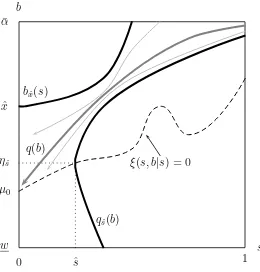
> 0. Thus, Assumption 5(b) is met. However, Assumption 5(a) fails. We illustrate this failure with Figure 2. The figure shows the function b(s) in this case along with its solution satisfying the boundary condition b(˜s10) = w.9 This extension of b(s) above w necessarily needs to
traverse a region, illustrated in gray, where ξ10(s, w|s)< 0. Therefore, there does not exist
a strictly increasing solution b(s) for all s >s˜10.
[Figure 2 about here.]
The main implication stemming from Example 2 concerns the possibilities and opportu-nities for inference in auction environments where bidders may be budget constrained. While there does not exist a good theory of inference and identification in auctions with budget constraints (and it is far beyond the scope of this study to develop one), changes in N are a common source of variation exploited in empirical auction studies.10 Fully exploiting this
variation in auctions with budget constraints may be problematic (or at best challenging) due to the qualitative differences of equilibrium bidding as the environment changes with
N. For example, for some values ofN (depending on the distribution of budgets and valua-tions), one would not be able to employ first-order conditions to fully characterize a bidder’s optimal bid. Much more research is required to develop precise conclusions and restrictions accounting for such concerns.
Public Signals
Suppose prior to bidding players observe the realization of some public signalS0. For
exam-ple, this signal may be some piece of information released non-strategically by the auctioneer. We begin by distinguishing two types of public signals that the bidders may observe.
Definition 2. A signalS0is said to be (strictly)value-relevant if for all (si,s−i),u(s0, si,s−i)
is (strictly) increasing in s0. S0 is said to be value-irrelevant if for all (si,s−i), u(s0, si,s−i)
is constant in s0.
9Precisely, we plot the solution of the inverse function—q(b)—as explained in the proof of Proposition 1. 10See Athey & Haile (2007) for a recent survey of identification in auction models. See Bajari & Horta¸csu
Definition 3. A signalS0 is said to beinformation-relevant if conditional onSi =si,S0 and
S−i are not independent. S0 is said to be information-irrelevant if conditional on Si = si, S0 and S−i are independent.
A signal that is value-relevant conveys information about the value of the item directly; its realized value is effectively a parameter of the bidder’s utility function. An information-relevant signal is correlated with other bidders’ private information. Therefore, it conveys additional information about others’ signals beyond the information contained already inSi. While nothing precludes a signal from being both value- and information-relevant—indeed, we consider this to be the norm—we will focus only on extreme cases where public signals are either value- or information-relevant, but not both. This dichotomy allows us to characterize the competing effects of information in the all-pay auction. Signals that are purely value-relevant encourage bidders to respond in the intuitive manner—“good news” will encourage uniformly more aggressive bidding. In contrast, high realizations of signals that are purely information-relevant are a discouragement leading some bidders to bid less.
Proposition 2. Suppose the conditions of Proposition 1 are satisfied and letw >0. Lets′
0 >
s0 be realizations of a public signal S0 observable to all bidders. Let β(s, w|s′0)[β(s, w|s0)] be
the equilibrium strategy in the all-pay auction when the public signal is high [low].
(a) If the public signal is value-relevant and information-irrelevant, thenβ(s, w|s′
0)≥β(s, w|s0).
(b) If the public signal is information-relevant and affiliated with players’ value-signals but is value-irrelevant, then there exists an ˆs > 0 such that for all s < sˆ, β(s, w|s′
0) ≤
β(s, w|s0).
Consider first the case of purely value-relevant information. Noting the preceding discus-sion, and viewings0as a parameter enteringuit is clear that our equilibrium characterization
remains the same with statements conditional ons0 replacing the unconditional statements.
An implicit assumption, of course, is that changes in s0 are sufficiently small to ensure (via
an appeal to continuity) that we maintain an equilibrium inM. The associated comparative static is intuitive.
In turning to information-relevant signals, we observe a different reaction. This conclusion is independent of the presence of budget constraints per se but is instead a general feature of the all-pay auction. The intuition is straightforward. Conditional on observing a high public signals′
0 bidderican infer that her opponent likely has a high signal and will in consequence
auction, discouraging her from bidding aggressively (recall, in an all-pay auction she must pay her bid irrespective of the outcome). In contrast, if the public signal also has a direct effect on a bidder’s value for the item, the resulting boost in expected payoff may be enough to counteract the discouragement effect.
3
The War of Attrition
Given that the first-price, second-price, and all-pay auctions have symmetric equilibria of the form β(s, w) = min{b(s), w}, a natural conjecture is that the war of attrition—the second-price, all-pay auction—also has an equilibrium in this class. In this section we extend our baseline model to accommodate this auction format as well. Many of the qualitative features of the all-pay auction’s equilibrium find natural analogues in the war of attrition. The major distinction is that under a very mild technical condition the war of attrition features a uniform amplification of bids following the introduction of budget constraints. In the all-pay auction, such an amplification was present generally only for a subset of types with intermediate valuations. The section concludes by noting the prospects for a revenue ranking between the all-pay auction and the war of attrition. Generally, such a ranking is not possible if both budget constraints and affiliated interdependent values are present.
We maintain our assumptions concerning the environment from Section 1. Again, bidders will simultaneously submit bids and the highest bidder will be deemed the winner. The winning bidder will make a payment equal to the second-highest bid. All losing bidders continue to incur a cost equal to their bid. Our static treatment of the war of attrition mirrors the treatment in Krishna & Morgan (1997). Therefore, we do not model the war of attrition as an extensive game where bidders sequentially submit additional (incremental) bids. Leininger (1991) and Dekel et al. (2006) consider such models with budget limits and perfect information. Extending our analysis in this direction would introduce many interesting complications such as the role of jump bidding in signaling valuationsand budget levels.
As in the case of the all-pay auction we first derive a differential equation that we will later prove characterizes equilibrium behavior. Suppose that all bidders j 6=i are following the bidding strategy β(s, w) = min{b(s), w} where b(s) : [0,1] → R+ is again a strictly
range of β(s, w), we extend its domain and range as follows. Let
ˆ
b(x) =
b(0) +x if x∈[−b(0),0)
b(x) if x∈[0,1] (13) ˆb(x) is also piecewise differentiable and strictly increasing. Then for all x ∈ [−b(0),1] the probability that maxj6=iβ(s, w) is less than ˆb(x) is given by
ˆ
H(x,ˆb(x)|s) =
N−1 X
k=0
N −1
k
G(ˆb(x))N−1−k(1−G(ˆb(x)))kFk(x|s). (14)
Since ˆb(x) is fixed, we can let ˆHˆb(x|s) ≡ Hˆ(x,ˆb(x)|s). ˆHˆb(x|s) is a cumulative distribution
function. Suppose its density is ˆhˆb(x|s). Using ˆHˆb(x|s) we can write the expected payoff of
a bidder of type (s, w) when she chooses to bid b(x)≤w and x >0, as
U(b(x)|s, w) =
N−1 X
k=0
γk(b(x))zk(x|s)−(1−Hˆˆb(x|s))b(x)
−
Z 0
−b(0)
(b(0) +y)ˆhˆb(y|s)dy− Z x
0
b(y)ˆhˆb(y|s)dy.
The first term is the same as in the all-pay auction. It is the expected benefit of winning the auction. The second term is the payment the bidder must make if she loses the auction. This is her own bid. The third and fourth terms define her payment when she wins the auction.
Proceeding analogously to the case of the all-pay auction, computing dxdU(b(x)|s, w)
x=s=
0 leads to the following differential equation:
b′(s) =
PN−1
k=0 γk(b(s))z′k(s|s)
1−Hˆˆb(s|s)−PkN=0−1γk′(b(s))zk(s|s)
.
Since ˆHˆb(s|s) = ˆH(s, b(s)|s) fors >0, we arrive at
b′(s) =
PN−1
k=0 γk(b(s))z′k(s|s)
1−Hˆ(s, b(s)|s)−PNk=0−1γ′
k(b(s))zk(s|s)
. (15)
private information and on the interaction between budgets and value-signals.
Suppose for the moment that b(s) < w, then (15) reduces to b′(s) = vN−1(s,s)fN−1(s|s)
1−FN−1(s|s) .
This again is the differential equation identified by Krishna & Morgan (1997) as describing a symmetric equilibrium of the war of attrition without budget constraints. In our notation, this strategy is
ω(s)≡
Z s
0
vN−1(y, y)fN−1(y|y)
1−FN−1(y|y)
dy. (16)
Recalling that lims→1ω(s) = ∞, leads us to anticipate an analogous development in our
model. Therefore, we strengthen Assumption 3 relating to the distribution of budgets as follows:
Assumption 6. For all w ≥ w in the support of G, G(w) admits a continuous, strictly positive density g(w).
Like in the all-pay auction, we will need a condition that limits the degree of affiliation among value-signals. The sufficient condition rendering ω(s) an equilibrium strategy in the absence of budget constraints is that
vN−1(·, y)fN−1(y|·)
1−FN−1(y|·)
: [0,1]→R (17)
is nondecreasing. Assumption 7 generalizes this condition to our setting.
Definition 4. The value ˜σ∈[0,1) is the unique solution to ω(˜σ) = w.
Assumption 7. Let qk(x, w|s) = γk(w)(1−Fk(x|s))
PN−1
n=1 γn(w)(1−Fn(x|s)). Define the function
Φ(x, w|s) =
N−1 X
k=1
qk(x, w|s)
vk(s, x)fk(x|s) 1−Fk(x|s)
. (18)
For all (x, w)∈[˜σ,1)×[w,w¯), Φ(x, w|·) : [0,1]→R is nondecreasing.
Assumption 8. Let qk(x, w|s) = γk(w)(1−Fk(x|s))
PN−1
n=1 γn(w)(1−Fn(x|s)). Define the function
Ξ(x, w|s) =
N−1 X
k=1
qk(x, w|s)
1− kg(w)
1−G(w)
zk−1(x|s)−zk(x|s)
1−Fk(x|s)
. (19)
Ξ(x, w|s) satisfies the following properties:
(a) For all σ˜ ≤ s < 1, ∃ws ∈ [w,w¯) such that w < ws =⇒ Ξ(s, w|s) < 0 and w ∈
(ws,w¯) =⇒ Ξ(s, w|s)>0.
(b) If σ >˜ 0, there exists ǫ >0 such that for all s∈(˜σ−ǫ,σ˜+ǫ), Ξ(s, w|s)>0. (c) For all (x, w)∈[˜σ,1)×[w,w¯), Ξ(x, w|·) : [0,1]→R is non-increasing.
Assumptions 8(a) and 8(b) fulfill the same role as Assumptions 5(a) and 5(b) in the all-pay auction. They ensure that there exists an increasing solution to the differential equation (15) in the appropriate range of values. The underlying intuition is also the same. Assumption 8(c) is particular to the war of attrition. The analogous requirement in the all-pay auction was implied by Assumption 4.11 In the war of attrition, we must impose
this condition explicitly since conditional on a given bid β(s, w), the expected payment of a bidder is a nontrivial function of (s, w). This contrasts with the all-pay auction where a bid ofβ(s, w) is associated with a certain payment of exactly that amount irrespective of (s, w). Some simplifications of Assumption 8 are possible in special cases of interest. For exam-ple, Assumption 8(c) is satisfied automatically if value-signals are independent. Likewise, if
N = 2, the following lemma is simple to confirm.
Lemma 2. SupposeN = 2. Then Assumption 1 implies Assumption 8(c).
Turning to the equilibrium characterization in the war of attrition, Proposition 3 identifies sufficient conditions for the existence of an equilibrium in the class M. The equilibrium strategy resembles the equilibrium of the all-pay auction. Low value-signal bidders will follow the usual no-budget-constraints equilibrium strategy. Only for bids above w will the change in marginal incentives introduced by budget constraints modify equilibrium behavior. Unlike the all-pay auction, bidders with sufficiently large value-signals will desire to expend an arbitrarily large (but feasible) amount in equilibrium.
11The analogous assumption in the all-pay auction would be that for all (x, w)
∈ [0,1) ×[0,α¯),
Proposition 3. Suppose Assumptions 1, 2, and 6–8 hold. Then there exists a symmet-ric equilibrium in the war of attrition of the form β(s, w) = min{b(s), w}. The function
b(s) : [0,1)→[0,w¯] is defined as:
b(s) =
ω(s) s <σ˜
b1(s) s ∈[˜σ,σˆ)
¯
w s >σˆ
(20)
whereb1(s) : [˜σ,σˆ)→ [w,w¯)is a strictly increasing, absolutely continuous function, such that
(a) b1(˜σ) = inf{w > w: Ξ(˜σ, w|σ˜)>0};
(b) lims→σˆ−b1(s) = ¯w; and,
(c) For almost every s, b′
1(s) =
PN−1
k=0 γk(b1(s))z′k(s|s)
1−Hˆ(s,b1(s)|s)−Pk=0N−1γk′(b1(s))zk(s|s).
Remark 2. We leave b(s) not defined ats = ˆσ. It can assume any value without affecting the equilibrium properties of this strategy profile. If ¯w <∞we could setb(ˆσ) = ¯wand make
b(s) continuous.
The following example illustrates an equilibrium strategy profile in the war of attrition. Occasionally, closed form expressions for the equilibrium strategy are available.
Example 3. SupposeN = 2 and that value-signalsSi i.i.d.∼ U[0,1]. Letu(si, sj) = (si+sj)/2 and suppose budgets follow the cumulative distribution G(w) = 1 −e−(w−w) on [w,∞).
Choose w=−7 20+ log
20 13
≈0.081. With these parameters, our equilibrium strategy in the war of attrition isβ(s, w) = min{b(s), w}where
b(s) =
−s−log(1−s) if s≤ 7 20 Rs
7 20
4y
3(y−1)2dy+w if s > 207
For s >7/20, we can integrate the above expression to see that
b(s) = 1040(s−1) log(1−s) + 1820(s−1) log
20 13
−1873s+ 833 780(s−1) . For comparison, Figure 3 presents the functions b(s) and ω(s) = −s−log(1−s).
As seen in Example 3, bidders with a value-signal of only 0.65 desire to commit to a bid greater than 1, which is the maximum possible value of the available prize. Such “overbidding” is a particular feature of the war of attrition (Albano, 2001). The effect of budget constraints is to amplify this phenomenon further. The following corollary formalizes this observation.
Corollary 2. Suppose the conditions of Proposition 3 hold and let w >0. (a) lims→σ˜+b′(s)>lims→σ˜−b′(s) = lims→σ˜−ω′(s).
(b) If fk(s|s)
1−Fk(s|s) ≥
fN−1(s|s)
1−FN−1(s|s) for all k.
12 Then for all s, b(s)≥ω(s).
Although the sufficient conditions supporting the equilibrium in the war of attrition are more restrictive, the equilibrium enjoys similar comparative statics. Again, the equilibrium strategy identified here will converge to the equilibrium in an environment without budget constraints if the constraints are relaxed. However, noting Corollary 2(b), a sufficient relax-ation of budget constraints will lead to an ordering of equilibrium strategies, much like in the second-price auction. Additionally, the same bidder-level comparative statics apply concern-ing information revelation. The distinction between value-relevant and information-relevant public signals continues to be important in appreciating a bidder’s equilibrium reaction to public information.
Proposition 4. Suppose the conditions of Proposition 3 are satisfied and letw >0. Lets′
0 >
s0 be realizations of a public signal S0 observable to all bidders. Let β(s, w|s′0)[β(s, w|s0)] be
the equilibrium strategy in the all-pay auction when the public signal is high [low].
(a) If the public signal is value-relevant and information-irrelevant, thenβ(s, w|s′
0)≥β(s, w|s0).
(b) If the public signal is information-relevant and affiliated with players’ value-signals but is value-irrelevant, then there exists an ˆs > 0 such that for all s < sˆ, β(s, w|s′
0) ≤
β(s, w|s0).
3.1
Comparing of the All-Pay Auction and the War of Attrition
We conclude our investigation with a brief comparison of the two auction formats. Naturally, we restrict attention to environments where the all-pay auction has an equilibrium of the formβA(s, w) = min{bA(s), w} ∈ Mand the war of attrition has an equilibrium of the form
12The condition is satisfied, for example, whenS
i i.i.d.
βW(s, w) = min{bW(s), w} ∈ M. Our first comparison considers an ordering of the bidding strategies.
Proposition 5. If w >0 then βW(s, w)≥βA(s, w) for all (s, w). Moreover, bW(s)> bA(s)
for all s >0.
Noting Proposition 5, we can employ the arguments in Che & Gale (1998) and also outlined in Krishna (2002) to conclude that the all-pay auction will be more efficient on average than the war of attrition when preferences are reflective of the ordering of bidder’s value-signals.13
We close with a discussion of revenue comparisons between the two formats. There does not exist a general revenue ranking between the war of attrition and the all pay auction in the presence of budget constraints and affiliated valuations. One can draw this conclusion by documenting the results in extreme cases. First, suppose that budget constraints are very lax. For example, suppose budgets are distributed according to the exponential distribution with a mean that is arbitrarily large. Since valuations are bounded the equilibrium bids sub-mitted in both formats are essentially those subsub-mitted in the case of a no-budget constraints situation. In this case, it is known that in the presence of value interdependence the war of attrition will revenue dominate the all-pay auction (Krishna & Morgan, 1997).
When budget constraints are more meaningful, and they constrain bidders with non-vanishing probability, the all-pay auction can generate more revenue. Consider the following case. Suppose there are two bidders and value signals are distributed independently according to the uniform distribution. Suppose budget constraints follow the exponential distribution
G(w) = 1−e−(w−w) on [w,∞). Choose w= log(10 3)−
7
10 ≈0.5039. Finally, assume bidders
have private values: ui(si, sj) =si.
In this situation, budget constraints are irrelevant in the case of the all-pay auction. The equilibrium strategy is βA(s, w) = min{bA(s), w} where bA(s) = s22. The expected revenue in the all-pay auction is RA= 13.
Since the bidding strategy in the war of attrition is not bounded, the introduced budget constraints will directly affect the equilibrium strategy. It is straightforward to show that the equilibrium bidding strategy isβW(s, w) = min{bW(s), w} where
bW(s) =
s if s < 7
10 Rs
7 10
y
(y−1)2dy+ log(103)−107 if s≥ 107
13For alls= (s1, . . . , s
When s > 107, we can write bW(s) in closed form as
bW(s) = s log
1000 27
−10+ 7 + log(27)−3 log(10) 3(s−1)
+ log
10 3 −
10 3 s
− 7
10. A direct calculation for the revenue in this case now gives
RW = 9
250 5 log
10 3
−1−5e20/3
Z ∞
20 3
e−t t dt
!
+ 581 + 270 log(3)−270 log(10) 1500 .
The terms in RW are straightforward to approximate accurately to conclude that RW <
0.327. In this example the impact on revenue following the introduction of budget constraints is very slight for two reasons. First, only about 30% of bidders in the war of attrition are somehow directly impacted by the budget constraint. Additionally, those who are impacted adjust their bidding upward (Corollary 2) which partially ameliorates the revenue decline. This adjustment is not sufficient to preclude a strict revenue decline.
While tractability has guided our discussion of revenues towards comparisons of extreme scenarios, its conclusions apply more generally. It is clear that we can modify our final example by perturbing the distribution of budgets slightly such that it has full support on [0,∞) without changing the conclusion. Similarly, one can perturb the distribution of value-signals such that they are strictly but “slightly” affiliated while maintaining the strict difference in expected revenues. For example, consider the distribution h(s1, s2)∝K+sisj
on [0,1]2 and let K be very large. Finally, one can introduce strict value interdependence
A
Proofs from Section 2 (All-Pay Auction)
Proof of Proposition 1
The proof of Proposition 1 has several steps which we present as a sequence of lemmas. Proofs of additional minor lemmas, referenced throughout, are in Appendix C.
We first establish the existence of the functionb(s). We begin by identifying a useful bound in Lemma 3. If the distribution of budgets satisfies this bound our main differential equation, equation (9), will have increasing solutions for allb(s) sufficiently large. With a fixed point argument, Lemma 4 shows that the introduction of this bound (which has a self-referential definition) is consistent with our maintained assumptions.
Considering only distributions of budgets that satisfy the derived bound and whose cumulative distribution function is continuously differentiable, we proceed to the define the function b(s). By restricting the distribution of budgets in the manner that we have, we can guarantee thatb(s) can be defined for all ∈[0,1] and that it is nondecreasing throughout this entire domain. Throughout this step we frequently work with the inverse of b(s). This is a common technique in analysis of equilibria in auctions.14
Having definedb(s) in a satisfactory manner for all [0,1], we establish that it is indeed bounded from above by ¯α. Arriving at this conclusion beforehand is generally not possible. Our argument at this step requires b(s) to be defined for all s ∈ [0,1] and satisfying all possible contingencies with regards to its definition necessitated the restrictions we imposed on G(·) in the preceding discussion.
As a final step we observe that since b(s) is bounded by ¯α the modification of the distribution of budgets forw >α¯ was unnecessary. Gdoes not need to satisfy the introduced bound nor does it have to be differentiable in this upper range of values.
Remark 4 and Lemma 11 concludes the proof by confirming that β(s, w) = min{b(s), w} is indeed a symmetric equilibrium strategy.
Throughout the discussion, we suppose Assumptions 1–5 are satisfied.
Defining a Special Class of Distributions
Lemmas 3 and 4 serve to define a special class of distribution functions for budgets. The key con-clusion from these lemmas is that when player’s budgets are distributed according to a distribution that meets the conditions of Lemma 3, then the differential equation (9) will have nondecreasing solutions in the range of values relevant for our problem.
Lemma 3. Suppose G(w) meets Assumptions 2, 3, and 5. Additionally, suppose
1. G(w) is continuously differentiable on [w,w¯) with a strictly positive derivative g(w).
2. For all w∈[¯α,w¯), G(w) satisfies the bound
g(w)
g(¯α) ≤
sups∈[˜s,1]PkN=0−2 Nk−2G(¯α)N−2−k(1−G(¯α))k[z
k(s|s)−zk+1(s|s)]
sups∈[˜s,1]PkN=0−2 Nk−2G(w)N−2−k(1−G(w))k[z
k(s|s)−zk+1(s|s)]
. (21)
Then the function ξ(x, w|s) defined in (11) exists for all w∈[w,w¯) and is continuous. Moreover, for alls≥˜s, ∃ws∈[w,α¯)such thatw < ws =⇒ ξ(s, w|s)<0 andw∈(ws,w¯] =⇒ ξ(s, w|s) >0.
Proof of Lemma 3. Thatξ is well defined for all w ∈[w,w¯) is a consequence of the additional differentiability assumption onG(w). We therefore only need to verify the single crossing condition. Suppose s ≥ ˜s. From Assumption 5(a), there exists ws < α¯ such that for all w ∈ (ws,α¯],
ξ(s, w|s) >0. Therefore, it is sufficient to establish that if (21) is satisfied then ξ(s, w|s) >0 for
w >α¯.
Using Lemma 14 and since ξ(s,α¯|s) > 0 for all s ∈ [˜s,1], we can write ∆zk(s) = zk(s|s)−
zk+1(s|s) to derive the following implications:
∀s∈[˜s,1], ξ(s,α¯|s)>0
=⇒ ∀s∈[˜s,1], g(¯α)
N−2
X
k=0
N −2
k
G(¯α)N−2−k(1−G(¯α))k∆zk(s)<
1
N −1
=⇒ g(¯α) sup
s∈[˜s,1]
N−2
X
k=0
N −2
k
G(¯α)N−2−k(1−G(¯α))k∆zk(s)<
1
N−1
=⇒ g(w) sup
s∈[˜s,1]
N−2
X
k=0
N −2
k
G(w)N−2−k(1−G(w))k∆zk(s)<
1
N −1, ∀w >α¯
=⇒ ∀s∈[˜s,1], g(w)
N−2
X
k=0
N−2
k
G(w)N−2−k(1−G(w))k∆zk(s)<
1
N −1, ∀w >α¯
Thus, for all w > ws and ˜s≤s,ξ(s, w|s)>0.
Lemma 4. Suppose G(w) is any distribution satisfying Assumptions 2, 3, and 5. Then there exists a cumulative distribution function G˜(w) with support [w,w˜), w >˜ α¯, such that G˜ meets the conditions of Lemma 3 and for all w≤α¯, G˜(w) =G(w).
Proof of Lemma 4. LetG(w) be any cumulative distribution function meeting Assumptions 2, 3, and 5 with densityg(w) defined for [w,α¯]. For any cumulative distribution functionF: [0,∞) → [0,1] define the functional
δ(F, w) = sup
s∈[˜s,1]
N−2
X
k=0
N−2
k
F(w)N−2−k(1−F(w))N−2−k[zk(s|s)−zk+1(s|s)] (22)
Note that for any F, δ(F, w) ≤ sups∈[˜s,1]z0(s|s) ≤ 1 and δ(F, w) ≥ minksups∈[˜s,1]zk(s|s) −
zk+1(s|s)≡D >0.
LetKbe the set of all continuous, nondecreasing functionsF: [¯α,∞)→[0,1] such thatF(¯α) =
G(¯α),F(w) = 1 for allw >α¯+g(¯α1−)δG(G(¯α(¯α))), and |F(w)−F(w′)| ≤ g(¯α)δ(G(¯α))
D |w−w′|. The set K is
equicontinuous and uniformly bounded; hence, compact. It is also convex. Consider the mappingF0−→Λ F1 defined by
F1(w) = Λ(F0)≡min
1, G(¯α) +
Z w
¯
α
g(¯α)δ(G,α¯)
δ(F0, t)
(To preclude confusion, F0 and F1 do not necessarily correspond to the distributions defined in
(3).) We record several facts about Λ.
1. Λ(K)⊂ K. To see this conclusion note that Λ(F0) =F1(w) is nondecreasing, continuous and
when w >α¯ yetF(w)<1,
F1(w) =G(¯α) +
Z w
¯
α
g(¯α)δ(G,α¯)
δ(F0, t)
dt
≥G(¯α) +
Z w
¯
α
g(¯α)δ(G,α¯)dt
=G(¯α) + (w−α¯)g(¯α)δ(G,α¯)
SinceF1 is bounded above by 1,F1(w) = 1 whenw >α¯+g(¯α1−)δG(G(¯α(¯α))). To verify the Lipschitz
condition, note thatg(¯α)δδ((GF(¯α))
0,t) ≤
g(¯α)δ(G(¯α))
D .
2. Λ is continuous. Define M = maxksupw∈[G(¯α),1]|dwd (wN−2−k(1 −w)k)|. Then, M < ∞.
TakingF0, F1∈ K, we see that
g(¯α)δ(G,α¯)
δ(F0, w) −
g(¯α)δ(G,α¯)
δ(F1, w)
≤ g(¯α)δ(G(¯α))
D2 |δ(F0, w)−δ(F1, w)|
≤ sup
s∈[0,1]
z0(s|s)
N−2
X
k=0
N−2
k h
F0(w)N−2−k(1−F0(w))k−F1(w)N−2−k(1−F1(w))k
i
≤ sup
s∈[0,1]
z0(s|s)(N −1)M|F0(w)−F1(w)|.
The continuity of Λ in the sup-norm follows immediately.
Since Λ is a continuous self-map acting on a compact, convex set, it has a fixed point, say ˜F = Λ( ˜F). With this function define the distribution function ˜G(w) as follows:
˜
G(w) =
(
G(w) ifw≤α¯ ˜
F(w) ifw >α¯ (23)
It is simple to verify that ˜G has the properties claimed by the Lemma. In particular, its density function ˜g(w) is continuous and it satisfies the required bound with equality forw≥α¯.
Defining the Function b(s) (Case of w >0)
composed of three components:
b(s) =
α(s) s∈[0,s˜)
b1(s) s∈[˜s,s¯1]
b2(s) s∈(¯s1,1]
(24)
The relationship between components is illustrated in Figure 4. α(s) is defined as in (10). We defineb1 as the inverse of the solution of the differential equation q′(b) =ψ(b, q(b)),
ψ(b, s) = 1−
PN−1
k=0 γk′(b)zk(s|s)
PN−1
k=1 γk(b)zk′(s|s)
, (25)
subject to the boundary condition q(w) = ˜s. Moreover, we restrictq(b) to the region [w,α¯]×[0,1]. As we show, this solution will be a strictly increasing function q: [w,¯b1]→ [0,1]. There are now
two possible cases:
1. If, as illustrated in Figure 4, ¯b1= ¯α (and thus q(¯b1) = ¯s1 <1), we defineb2(s) as the strictly
increasing solution tob′2(s) =ρ(s, b2(s)),
ρ(s, b) =
PN−1
k=1 γk(b)z′k(s|s)
1−PNk=0−1γk′(b)zk(s|s)
, (26)
meeting the boundary conditionb2(¯s1) = ¯α.
2. If instead ¯b1 <α¯, we argue thatq(¯b1) = ¯s1= 1. In this case the definition of b2(s) above not
needed.
Whatever the case we are able to define a functionb: [0,1]→[0,w¯] by (24). We have separated the definition of b(s) into the components b1 and b2 to be able to identify solutions to (25) and (26).
Bothψ andρ may be undefined in certain regions of [˜s,1]×[w,w¯]; however, in a region where one fails the other does not.
[Figure 4 about here.]
Lemma 5 (Case 1: w > 0). Suppose w >0 and that G(w) satisfies the hypotheses of Lemma 3. Consider the function
ψ(b, q) = 1−
PN−1
k=0 γk′(b)zk(s|s)
PN−1
k=1 γ(b)zk′(s|s)
defined for (b, s)∈[w,α¯]×[0,1]. Then there exists a strictly increasing function q: [w,¯b1]→[˜s,1]
which is a solution to the differential equation q′(b) = ψ(b, q(b)) satisfying the boundary condition
q(w) = ˜s.
Proof of Lemma 5. It is simple to verify thatψ(b, s) is continuous on [w,α¯]×[ǫ,1] for all 0< ǫ <˜s. Thus, the boundary value problem has a solution in this restricted domain. Letq(b) : [w,¯b1]→[0,1]
be the maximal solution in the sense of largest domain.15