Some Explicit Results for the Distribution Problem of Stochastic Linear Programming

(1)

http://www.scirp.org/journal/ojop ISSN Online: 2325-7091 ISSN Print: 2325-7105

Some Explicit Results for the Distribution

Problem of Stochastic Linear Programming

Afrooz Ansaripour

1

, Adriana Mata

2

, Sara Nourazari

3

, Hillel Kumin

4

1_{Penn State University, State College, PA, USA} 2_{CAF Development Bank, Caracas, Venezuela}

3_{California State University at Long Beach, Long Beach, CA, USA} 4_{University of Oklahoma, Norman, OK, USA}

Abstract

A technique is developed for finding a closed form expression for the cumulative distribution function of the maximum value of the objective function in a stochastic linear programming problem, where either the objective function coefficients or the right hand side coefficients are continuous random vectors with known probability distributions. This is the “wait and see” problem of stochastic linear programming. Explicit results for the distribution problem are extremely difficult to obtain; indeed, previous results are known only if the right hand side coefficients have an exponen-tial distribution [1]. To date, no explicit results have been obtained for stochastic c, and no new results of any form have appeared since the 1970’s. In this paper, we ob-tain the first results for stochastic c, and new explicit results if b an c are stochastic vectors with an exponential, gamma, uniform, or triangle distribution. A transforma-tion is utilized that greatly reduces computatransforma-tional time.

Keywords

Stochastic Linear Programming, The Wait and See Problem, Mathematics Subject Classification

1. Introduction

Consider the linear programming problem,

( )

Max z x =cx (1)

( )

. : ,

s t A I x=b (2)

0

x≥ (3)

How to cite this paper: Ansaripour, A., Ma- ta, A., Nourazari, S. and Kumin, H. (2016) Some Explicit Results for the Distribution Problem of Stochastic Linear Programming. Open Journal of Optimization, 5, 140-162. http://dx.doi.org/10.4236/ojop.2016.54014

Received: October 30, 2016 Accepted: December 27, 2016 Published: December 30, 2016

(2)

where c is an 1×

(

m n+

)

vector whose jth component is cj (where, cj =0, for

j>n) and b is an m×1 vector whose i_th component is bi, A=

( )

aij is an m n×

matrix, I is an m m× identity matrix and x is an

(

m n+ ×

)

1 vector. Further assume that b and c are random vectors with joint density functions f b

( )

and g c

( )

re-spectively. Next, consider the value of z x

( )

by first observing the vector b or the vec-tor c and then solving (1)-(3). This paper is interested in finding explicit expressions for the distribution of maxz x

( )

if either b or c is random. This is called the distribution problem of stochastic linear programming.

Early work on the distribution problem can be found in Babbar [2], Bereanu [3] [4]

[5] [6] [7], Hsia [8], Prekopa [9], Sengupta, Tintner, and Millham [10], Sengupta,

Tintner, and Morrison [11], and Wets [12]. For additional references, see the biblio-graphies by Stancu-Minasian [13] and Van Der Vlerk [14]. Application of the distribu-tion problem can be found in the areas of agriculture [15] and economic planning [10],

[11]. Explicit results for the distribution of maxz x

( )

are very difficult to obtain; in-deed, most analyses rely on approximation techniques or simulation. (See, for example, Bracken and Soland [16], Sarper [15], or Dempster [17]). Bereanu [3] discovered that under certain assumptions, the sample space of the random coefficients allows a parti-tion into non-overlapping sets, called decision regions, such that a basis of the linear programming problem can be assigned to each of the sets, and this basis remains op-timal for all of its sample points. Ewbank, et al. [1] extended this theory using a Jaco-bian transformation to simplify the computational analysis. To date, we believe that an explicit expression for the distribution of maxz x

( )

has only been obtained for sto-chastic b [1], and no explicit results have been obtained for stochastic c. In addition, no explicit results have been obtained for non-exponential distributions. In this paper, we obtain new explicit results for exponential, uniform, gamma, and triangle distributions with b or c random. These are the first explicit results for the case in which c is random.

2. Theory

Following [1], consider the linear programming problem (1)-(3). Let

(

1, ,

)

i i i

B m

x = x  x

be the vector of basic variables corresponding to the ith basis, and Bi is the m m× basis matrix whose columns are the columns of

(

A I,

)

corresponding to the elements of i

B

x . Let ciB =

(

c₁i,,cim

)

be the vector of coefficients of the basic variables in ith basis and let aj be the jth column of

(

A I,

)

corresponding to cj. Also,

{

i is a basic variable

}

i j

D = j x and Ei =

{

k xki is a nonbasic variable

}

. Bi is an op-timal basis if

1

0

i

B i j j

c B a− −c ≥

For all

1, ,

j=  m+n (4)

and is feasible if

1 0 i

(3)

For the case in which the b vector is random, let the probability space be defined by the m-tuple

(

b1,,bm

)

. Bereanu discovered that there exist non-overlapping regions

( )

{

1

}

0 for all 1, ,

i i

j

S = b B b− ≥ j=  m (6)

where

(

_k _l

)

0 for

P S ∩S = k≠l (7)

Thus,

( )

{

}

( )

{ }

Pr Pr i Pr i

i

z x ≤ ∅ = z x ≤ ∅ S S

 

 

∑

  (8)

Now, let

{

}

i i

V = b b∈S

Since

{ }

( )

1

Pr d

i

m

i i i

V

S =

∫ ∫

 f b

∏

₌ b (9)

Then

( )

{

}

{

( )

}

{ }

Pr z x ≤ ∅ ∩ Si =Pr z x ≤ ∅Si Pr Si (10)

( )

{

}

{

( )

}

{ }

Pr z x ≤ ∅Si =Pr z x ≤ ∅ ∩ Si Pr Si (11)

( )

{

}

( )

1

Pr d

i i B B i

m

i i i

c x V

z x S f b ₌ b

 ≤∅ ∩

 

≤ ∅ ∩ =

 

 

∫ ∫



∏

(12)

Thus,

( )

{

}

{

( )

}

Pr z x ≤ ∅ =

∑

iPr z x ≤ ∅ ∩ Si (13)

Now, consider the case in which only the c vector is random. Let the probability space C be defined by the n-tuple c=

(

c1,,cn

)

. Bereanu [3] found that the space C is partitioned by the sets:

{

1

}

0 for all such that

i i i

i B i j j j

T = c c B a− −c ≥ j x ∈E (14)

where i refers to the i_th basis. Further the set of points

{

i 1 _{0 for all} i

}

B i j j

c c B a− −c = j∈E is of probability measure zero if the joint density

function of i is continuous. Points in this set are such that alternate optimal basis give the same value of z x

( )

. Also,

{

}

Pr Tk∩Tl =0 for k≠l (15)

Thus,

( )

{

}

{

( )

}

( )

{ }

Pr z x ≤ ∅ =

∑

i Prz x ≤ ∅ ∩ Ti =

∑

iPrz x ≤ ∅ TiPr Ti (16)

(4)

To evaluate the right-hand side of equation Equation (15) let Ui=

{

c c∈Ti

}

. By

de-finition

{ }

( )

1

Pr d

i

n

i i i

U

T =

∫ ∫

 f′ c

∏

₌ c (17)

Since

( )

{

}

( )

{ }

Pr z x ≤ ∅ ∩ Ti =Prz x ≤ ∅ TiPr Ti (18)

Then

( )

{

}

{

( )

}

{ }

Pr z x ≤ ∅Ti =Pr z x ≤ ∅ ∩ Ti Pr Ti (19)

where

( )

{

}

( )

1

Pr d

i i B B i

n

i i i

c x U

z x T f c ₌ c

 ≤∅ ∩

 

′ ≤ ∅ ∩ =

 

 

∫ ∫



∏

(20)

Thus, if only the c vector is random the distribution function of max z x

( )

can be found, in theory, by evaluating the integral in equation Equation (20). Given a basis Bi and sets Ui and Vi, the limits of the integral in Equation (12) and Equation (20) are the intersection of m or n hyperplanes (depending on whether the b vector or the c vector is stochastic). These limits are extremely difficult to obtain if the probability space has dimension greater than 3. Ewbank, et al., [1] developed a Jacobian transfor-mation that greatly simplifies the computation of the integrals.

In the case of stochastic b, Let

1 0 i

B b− ≥ (21)

By substituting for b we have:

(

1

)

B B b− = =b Br (22)

The probability that a basis G remains feasible is

( )

1d

m

i i

s

P=

∫ ∫

 f b

∏

= b (23)

where s is the set of b’s defined in Equation (20), and by substituting Equation (21) in

Equation (22), we have:

(

)

1

0

d m

r i i

r

P f Br J ₌ r

≥

=

_{∫∫ ∫}

_

∏

₍₂₄₎

where Jr is the Jacobian

[

]

det

r k i

J = ∂b ∂r

Because

( )

1

m

k k j kj j

b = Br =

∑

₌B r and ∂bk ∂ =ri Bki, this implies

[ ]

( )

det det

r ki

J = B = B (25)

(5)

3. Computational Results

The problems were run using the Mathematica software version 8.0.1.0 utilizing the supercomputer at the University of Oklahoma.

 _{CPUs: All compute nodes have dual Intel Xeon E5-2650 “Sandy Bridge” oct core 2.0} GHz CPUs; there is also one “fat node” with quad Intel Xeon E7-4830 “Westmere” oct core 2.13 GHz CPUs.

 RAM: Most of the compute nodes have 32 GB of 1333 MHz RAM and 23 with 64 GB of 1333 MHz RAM; the one “fat node” has 1 TB of 1066 MHz RAM, which is called large memory.

 _{Accelerators: There are 18 NVIDIA Tesla M2075 cards, for an aggregate of an} addi-tional approximately 9 TFLOPs double precision.

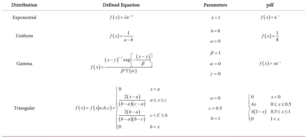
In order to compare the run times, four types of distributions were considered as shown in Table 1. The coefficients were randomly generated in small interval, because large intervals led to computational results that had results with coefficients of the or-ders of 1020 or larger.

3.1. Results for Stochastic b with Exponential Distribution

3.1.1. Problem 1

Case Case I. Stochastic Resource Vector. Ewbank’s model

A 1 1

1 2

 

 

 

B

{

b b1, 2}~ Exponential iid(λ=1)

C { }2,3

CDF

(

)

1

e 6 6e 0 6

0 0

∅ ∅

 _{− +} _{− ∅} _{∅ >}

 

 _{∅ <}



CDF Plot

(6)

Case Case I. Stochastic Resource Vector. Bereanu’s model

A 1 1_{1 2}

 

B

{

b b1, 2}~ Exponential iid(λ=1)

C { }2, 3

CDF

(

)

1

e 6 6e 0 6

0 0

∅ ∅

 _{− +} _{− ∅} _{∅ >}

 

 _{∅ <}



CDF Plot

[image:6.595.43.554.468.696.2]

Time 4.134 seconds.

Table 1. Equations of distribution.

Distribution Defined Equation Parameters pdf

Exponential ( ) e x

f x =λ −λ λ=1 ( ) ex

f x = −

Uniform f x

( )

1

a b = − 8 b= 0

a=

( )

1 8

f x =

Gamma _{( )} ( )

( )

1

exp x y

x

f x _α

γ β β α ∝−  −  − _− _   = Γ 1 β= 0 α= 0 γ=

( ) ex

f x =x −

Triangular ( )

(

)

( ) ( )( ) ( ) ( )( ) 0 2 , , 2 0 x a x a

a x c

b a c a

f x f x a b c

b a

c C b

b a b c

b x <   ₋  _{≤ ≤}  − −  = =  ₋

 _{< ≤}

 − −   <  0 a= 0.5 c= 1 b= ( ) 0 0

(7)

3.1.2. Problem 2

A

42 64 62 18 3 3 68 65 2 34 65 17 32 20 13 1 10 55 37 56 44 7 30 11

62 39 59 61 52 24 18 35 50 65 5 42

 

 

 

B {b b b b b b1, 2, ,3 4, ,5 6}~ Exponential iid(λ=1)

C {53, 57, 38, 7, 1, 32}

CDF

186 115 93

7 19 19

259 19

53 4

1126418971 174827706709 148007864405 1

126591405630e 334942876224e 89303808e 187191798507739 23288387

0 189486e

105177626880e 0

∅ ∅ ∅

∅ ∅

+ − −

+ − ∅ >

0

     

 _{∅ <}

 

CDF Plot

Time 1335.08 Seconds.

A

42 64 62 18 3 3 68 65 2 34 65 17 32 20 13 1 10 55 37 56 44 7 30 11

62 39 59 61 52 24 18 35 50 65 5 42

 

 

 

B {b b b b b b1, 2, ,3 4, ,5 6}~ Exponential iid(λ=1)

C {1, 2, 3, 2, 1, 1}

(8)

3.1.3. Problem3

A

13 69 56 45 23 39 34 4 38

30 65 8 51 29 59 65 54 18

30 20 53 5 46 52 55 32 1

65 45 4 41 43 50 41 5 54

3 31 31 46 19 49 2 64 2

26 52 67 13 27 55 59 0 63

13 55 31 35 46 29 23 40 34

55 16 40 37 62 48 34 21 14

7 21 14 32 55 66 47 45 34

 

 

 

B

{

b b b b b b b b b1, 2, ,3 4, 5, 6,, 7, ,8 9

}

~Exponential iid(λ=1)

C {63, 58, 33, 49, 50, 64, 47, 70, 40}

CDF

304 360

33 47

257 365

40 58

305 49

923512167204243 4587824269069469 1

112421428303294292 722317922166417500

1829039266689190654 727938601434779113 2336758228034180379 410788623816360000

1665192956 139

e e

e

− ∅ − ∅

− ∅

+ −

− −

−

55 14

242 63

14540635702595879 4020125 398109809908800

264776529949169098094

0 7094601260302987937

0 0

e

− ∅

− ∅ 

       

 ₊

 

− ∅ >

∅ < 

   

CDF Plot

(9)

3.2. Results for Stochastic b with Uniform Distribution

3.2.1. Problem 1

A _1 1_{1 2}_

B

{

b b1, 2}~ Uniform 0,8( )

C { }2, 3

CDF

( )

(

2

)

480 11

0 12 460

1

256 96 3 12 16 512

1 16 0 0

B

 − ∅ ∅ _{< ∅ <}

 

 ₋ _{+ ∅ − ∅} _{< ∅ <}

 

∅ > ∅ < 

 

CDF Plot

Time 1.36 Seconds.

A 1 1

1 2

 

 

 

B

{

b b1, 2}~ Uniform 0,8( )

C { }2, 3

CDF

( )

(

2

)

480 11

0 12 460

1

256 96 3 12 16 512

1 16 0

B − ∅ ∅

< ∅ <

− + ∅ − ∅ < ∅ <

∅ >

0

      

 _{∅ <}

(10)

Continued

CDF Plot

Time 1.36 Seconds.

3.2.2. Problem 2

A

2 6 25 26 17 22 39 51 42

 

 

 

B

{

b b b1, 2, 3}~ Uniform 0,8( )

C {4, 3, 46}

CDF

(

2

)

2 3

1472736 78775 9299 32

0

460 39

46970460160 5987642931648 461528402256 11478091905 32 184

24705054176256 39

B ∅

∅

∅ − + + ∅

− < ∅ <

− + − ∅ + ∅ _{< ∅ <}

21 184 1

21 0

∅ >

0

        

 _{∅ <}



CDF Plot

(11)

3.2.3. Problem 3

A

4 10 3 5 1 4 5 5 10 6 4 4

2 8 8 5 1 5 7 9 5 2 8 3 2 6 4 8 1 2 8 6 7 6 8 6

                   

B

{

b b b b b b1, 2, ,3 4, 5, 6}~ Uniform 0,8( )

C {10, 2, 2, 9, 4, 4}

CDF

2 3

4 5

(94681969459200000 5187191675120000 623227239936000 88202659881600 371504185344000000

( 365032235188 51324519043

371504185344000000 ∅ ∅ ∅ − − ∅ + ∅ − ∅ + ∅ + 2 3

4 5 6

0 4

819350510400000 6671233548000000 588214667070000 4558298004000 ) 23219011584000000

214304599260 118583281368 1973181073

2319011584000000

∅

< ∅ <

− + − ∅ + ∅

∅ − ∅ + ∅

+

2

3 4 5

4 9

346924362544798400000 421027877219066400000 56208803310069330000 911852659408896000000

3814862723932876000 138065723884320600 2514521036736408 1802708402

∅

< ∅ ≤

− + − ∅

∅ − ∅ + ∅ −

+ 6

2 3

4 5 6

3513

9 10 911852659408896000000

2050268425803784192 1109709749741822976 255630745634538240 31026699217604480 72948212752711680

2096997758693760 74945946698532 1107879173351 7294821275271168

∅

∅ _{< ∅ ≤}

− + ∅ − ∅

∅ − ∅ + ∅

+ 10 148

0 13

113

< ∅ <

148 0 ∅ ≥ 0                             ∅ <  CDF Plot

(12)

3.3. Results for Stochastic b with Gamma Distribution

3.3.1. Problem 1

A _1 1_{1 2}_

B bi~Gamma(∝=2,β=1 ,)i=1, 2

C { }2, 3

CDF

(

)

2 3

1

e 648 648e 648 207 26 0 648

0 0

−∅ ∅

 ₋ ₊ ₋ _{∅ −} _{∅ − ∅} _{∅ >}

 

 _{∅ <}



CDF Plot

Time 1.685 Seconds

A _1 1_{1 2}_

B bi~ Gamma(∝=2,β=1 ,)i=1, 2

C { }2, 3

CDF

(

)

2 3

1

e 648 648e 648 207 26 0 648

0 0

−∅ ∅

 ₋ ₊ ₋ _{∅ −} _{∅ − ∅} _{∅ >}

 

 _{∅ <}



CDF Plot

(13)

3.3.2. Problem 2

A

2 1 2 3 1 2

1 6 1

 

 

 

B bi~ Gamma(∝=2,β=1 ,) i=1, 2, 3

C {5, 3, 2}

CDF

(

)

8 8 22

2 3

3 3 15

2 3

e 65884500e 243e (243000 379225 157905 15972

125 54684 24519 91355 26620 6588400 0

0

− ∅ ∅ ∅

  ₋ ₊ _{∅ +} _{∅ +} _∅ 

 _ _



+ − + ∅ + ∅ + ∅ ∅ >

0

    

 _{∅ <}

  

CDF Plot

Time 16.44

A

2 1 2 3 1 2

1 6 1

 

 

 

B bi~ Gamma(∝=2,β=1 ,)i=1, 2, 3

C {5, 3, 2}

CDF

(

)

8 8 22

2 3

3 3 15

2 3

e 65884500e 243e (243000 379225 157905 15972

125 54684 24519 91355 26620 6588400 0

0

− ∅ ∅ ∅

  ₋ ₊ _{∅ +} _{∅ +} _∅ 

 _ _



+ − + ∅ + ∅ + ∅ ∅ >

0

    

 _{∅ <}

(14)

Continued

CDF Plot

Time 26.52

3.4. Results for Stochastic b with Triangle Distribution

Problem 1

A

3 3 1 3 3 1 1 3 2

 

 

 

B

{

1 2 3}

(

)

₍ ₎

0 0

4 0 0.5 , , ~ Triangular 0,1, 0.5

4 1 0.5 1 0 1

b

b b

b b b b

b b

b < 

 _{≤ ≤}



=  ₋ _{≤ ≤}



 _<



C {3, 2, 2}

CDF

2 4 6

2 3

4 5 6

1.222 1.4537 1.7222

8.2003 52.7154 133.976 164.267 0 0.5 105.386 33.8097 4.21528 0.5 1

13.4184 4

6.8

∅ + ∅ − ∅

− ∅ + ∅ − ∅ ≤ ∅ ≤

+ ∅ − ∅ + ∅ ≤ ∅ ≤

− + 2 3

4 5 6

2 3

4 5 6

147 49.5551 5.9317

24.9566 17.3611 3.6169 1 1.1 26.2336 116.715 208.42 198.495

106.337 30.3819 3.6169 11. 1

∅ − ∅ + ∅

+ ∅ − ∅ + ∅ < ∅ ≤

− + ∅ − ∅ + ∅

− ∅ + ∅ − ∅ < ∅ < .4

1 1.4 0 0





∅ ≥ ∅ < 

          

CDF Plot

(15)

3.5. Results for Stochastic c with Exponential Distribution

3.5.1. Problem 1

Case Case II. Stochastic Resource Vector. Ewbank’s model

A 5 4

10 3

 

 

 

C

{

} (1 2)

1, 2 ~ e

CC

C C +

B { }6, 5

CDF

13 3 2

2

5 2 3

35 2

1 e e e e 0 33 33

0 0

− ∅ − ∅ − ∅

− ∅

 + − − − ∅ >

 

 _{∅ <}



CDF Plot

Time 5.85 Seconds

Case Case II. Stochastic Resource Vector. Bereanu’s model

A 5 4

10 3

 

 

 

C

{

} (1 2)

1, 2 ~ e

CC

C C +

B { }6, 5

CDF

13 3 2

2

5 2 3

35 2

1 e e e e 0 33 33

0

− ∅ − ∅ − ∅

− ∅

 + − − − ∅ >

 

 _{∅ <}



CDF Plot

(16)

3.5.2. Problem 2

A

10 2 5

1 3 2 6 3 4

 

 

 

C

{

} (1 2 3)

1, 2, 3 ~ e

C C C

C C C + +

B {7, 6, 5}

CDF

13 17 15 12

5 7 7 7

7 5 2 2

5 6 3 3

23368 205 1757 7 49

e e e e

23205 3744 6120 69 132

30 e 49 9 53

e e e e 0

119 160 85 44 69 0

e

− ∅ − ∅ − ∅ − ∅

−∅ −∅

− ∅ − ∅ − ∅ −∅

+ − + +

+ + + − − − ∅ >

0

     

 ∅ <

 

CDF Plot

Time 34.991 Seconds

3.6. Results for Stochastic c with Uniform Distribution

3.6.1. Problem 1

A 1 1

2 1

 

 

 

C

{

C C1, 2}~ uniform 0,8( )

B {10,10}

CDF

2

19

0 12

3600

2 5 40

12

7 56 5600 3

5(832 176 5 40 88

3584 3 5

0 5 88

∅

 _{< ∅ <}

 

∅ ∅

− + − < ∅ <

 

 ₋ _{∅ + ∅}

− < ∅ <



 ∅ >

(17)

Continued

CDF Plot

Time 2.606 Seconds

A 1 1

2 1

 

 

 

C

{

C C1, 2}~ uniform 0,8( )

B {10,10}

CDF

(

)

2

19

0 12

3600

2 5 40

12

7 56 5600 3

5 832 176 5 40 88

3584 3 5

0 5 88

∅

 _{< ∅ <}

 

 _∅ _∅

− + − < ∅ <

 

 ₋ _{∅ + ∅}

− < ∅ <

 

∅ > 

CDF Plot

(18)

3.6.2. Problem 2

A

20 38 23 40 36 26 24 30 29

 

 

 

C

{

C C C1, 2, 3}~ uniform 0,8( )

B {27, 22, 29}

CDF

(

2

)

2 3

16898367744 1625159 45699175

0 6 54618872832

885527518720 219442583488 214078289688 8704702125 1096 6

5682385695744 165 88146918912 222

∅ − ∅ + ∅

< ∅ ≤

− + ∅ − ∅ + ∅ _{< ∅ ≤}

− +

(

)

2 3

257865280 24372051240 878254875 1096 232

577406648320 165 33 3 4893594112 2398313408 307856280 13171149 232 856

4001054720 33 11 1

∅ − ∅ + ∅ _{< ∅ ≤}

− + ∅ − ∅ + ∅

< ∅ ≤

111 856 0

∅ >

0

            

 _{< ∅}



CDF Plot

Time 105.144 Seconds

3.7. Results for Stochastic c with Gamma Distribution

3.7.1. Problem 1

A _1_{3 1}2_

C

{

} (1 2)

1, 2 ~ 1 2e

CC

C C C×C +

B { }3, 2

CDF

( ) ( )

(

) (

)

4

2 2 3 2

2 2

1

e 216e 72e 3 2 108e 2 3

216

+e 20 50 8 7 28 66 27 0

0 0

∅ ∅

− ∅ ∅

∅ 

 ₋ _{+ ∅ −} _{+ ∅}

 

 _{− ∅ − ∅ +} _{+ ∅ + ∅} _{> ∅}

  

 _{∅ <}

(19)

Continued

CDF Plot

Time 9.454 Seconds

A _2₂ 5₄_

C

{

} (1 2)

1, 2 ~ 1 2e

CC

C C C×C +

B { }3,1

CDF No Result

3.7.2. Problem 2

A

5 1 5 2 4 3 1 1 5

 

 

 

C

{

} { } (1 2 3)

1, 2, 3 ~ 1 2 3 e

C C C

C C C C×C ×C − + +

B { }3, 2

CDF

13 17

15e 12

5 7

e 7

7 5 2

5 6 3 2 3

23368 205e 1757e 7 49 e e 23205 3744 6120 69 132

30 e 49 9 53

e e e e e 0

119 160 85 44 69 0

− ∅ − ∅

− − ∅

∅

− ∅ − ∅ − ∅ −∅ −∅

− − + + +

+ + − − − ∅ >

0

    

 _{∅ <}

  

CDF Plot

(20)

3.8. Results for Stochastic c with Triangle Distribution

3.8.1. Problem 1

A 1 2

3 1

 

 

 

B

{

1 2 3}

(

) (

)

₍ ₎

0 0 4 0 0.5 , , ~ Triangular 0,1, 0.5 , ,

4 1 0.5 1

0 1

C

C C

C C C C f C a b c

C C C <   _{≤ ≤}  = =  ₋ _{≤ ≤}   _< 

C { }3, 5

CDF

4

2 3 4

0.38 0 0.75

0.027 0.27 1.026 1.53

0

.398 0.75 0.83

0.28 1.73 4.145 4.49 1.45 .083 1

∅ ≤ ∅ ≤

− + ∅ − ∅ + ∅ − ∅ ≤ ∅ ≤

2 3 4

.5

2.33 3.76 1.02 0.012 0.008 1.5 1.66

0.29 2.16 5.23 2.98 0.53 1.66 1.8

11.45 22.64 15.43 4.68

0.53 1.8 2.2

1

− + ∅ − ∅ − ∅ + ∅ ≤ ∅ ≤

− − ∅ + ∅ − ∅ − ∅ < ∅ ≤

− + ∅ − ∅ + ∅ − ∅ ≤ ∅ ≤

2.2

0 0

          ≤ ∅ 

 _{∅ <}



CDF Plot

Time 13.292 Seconds

3.8.2. Problem 2

A

2 1 5

2 2 4 2 1 4

 

 

 

C

{

1 2 3}

(

)

₍ ₎

0 0 4 0 0.5 , , ~ Triangular 0,1, 0.5

4 1 0.5 1

0 1

C

C C

C C C C

(21)

Continued

B {2, 2,1}

CDF

4

00.524755 2

1.32544 0 0.375

≤ ∅

∅ ≤ ∅ ≤

− 2 3 4

2 3 4

0.228579 0.16 1.12 0.623333 0.09875 15 2

0.271421 1.49333 2.45333 1.21593 0.197515 1 1.5

0.792255 3.16 4.45333 2.29926 0.426682 0.8 1

50.3958 333.907 91

8.213

− ∅ − ∅ − ∅ + ∅ ≤ ∅ ≤

− ∅ + ∅ − ∅ + ∅ ≤ ∅ ≤

− − ∅ − 2 3 4

5 6

4 5 6

1341.7 1098.47

478.271 86.5885 0.75 0.8

0.000798542 0.2133

49 1.66836 1.32544 0.4 0.75

0

∅ + ∅ − ∅

+ ∅ − ∅ < ∅ ≤

− − ∅ + ∅ − ∅ < ∅ ≤

0

              

 _{≥ ∅}



CDF Plot

Case Case II. Stochastic Resource Vector. Bereanu’s model

A

2 1 5 2 2 4 2 1 4

 

 

 

B

{

1 2 3}

(

)

₍ ₎

0 0 4 0 0.5 , , ~ Triangular 0,1, 0.5

4 1 0.5 1 0 1

C

C C

C C C C

C C

C < 

 _{≤ ≤}



=  ₋ _{≤ ≤}



 _<



C {2, 2,1}

CDF No Results

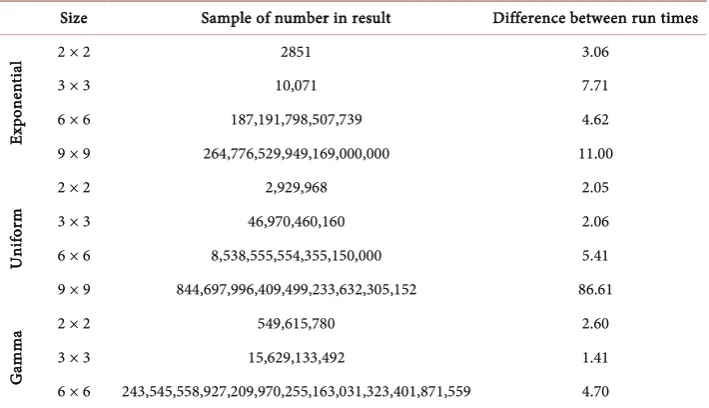
4. Computational Time Comparisons

The different distributions were solved using both Bereanu’s method and the Ewbank, Foote and Kumin transformation method to compare the two. Table 2 and Table 3

(22)

[image:22.595.199.554.89.293.2]

Table 2. Comparison between Bereanu and EFK method for case I.

Size Sample of number in result Difference between run times

Ex

po

nen

tial

2 × 2 2851 3.06

3 × 3 10,071 7.71

6 × 6 187,191,798,507,739 4.62

9 × 9 264,776,529,949,169,000,000 11.00

U

ni

fo

rm

2 × 2 2,929,968 2.05

3 × 3 46,970,460,160 2.06

6 × 6 8,538,555,554,355,150,000 5.41

9 × 9 844,697,996,409,499,233,632,305,152 86.61

G

am

ma 2 × 2 _{3 × 3} _{15,629,133,492}549,615,780 2.60 _1.41

6 × 6 243,545,558,927,209,970,255,163,031,323,401,871,559 4.70

Table 3. Comparison between Bereanu and EFK method for case II.

Dimention Bereanu’s Method EFK Method

Exponential

2 × 2 2.386 1.747

3 × 3 78.68 17.97

6 × 6 No Result 9176.28

Uniform 2 × 2 3.12 2.606

3 × 3 210.4 105.144

Gamma 2 × 2 No Result 11.544

3 × 3 No Result 115.004

Triangular 2 × 2 No Result 13.292

3 × 3 No Result 575.846

the EFK method substantially reduces the computational time. In addition, Bereanu’s method is not able to solve some larger sizes of the problem. All times are measured in seconds.

References

[1] Ewbank, J., Foote, B. and Kumin, H.A. (1974) Method for the Solution of the Distribution Problem of Stochastic Linear Programming. SIAM Journal on Applied Mathematics, 26, 225-238. https://doi.org/10.1137/0126020

[2] Babbar, M.M. (1975) Distribution of Solutions of a Set of Linear Equation with an Applica-tion to Linear Programming. Journal of the American Statistical Association, 50, 854-869.

https://doi.org/10.1080/01621459.1955.10501971

[image:22.595.196.554.323.493.2]

(23)

Dis-tribution of the Optimum and Applications. Journal of Mathematical Analysis and Applica-tions, 15, 280-294. https://doi.org/10.1016/0022-247X(66)90120-X

[5] Bereanu, B. (1966) On Stochastic Linear Programming II. Distribution Problems. Nonsto-chastic Technological Matrix. Revue Roumaine de Mathématique Pures et Appliquées, 11, 713-725.

[6] Bereanu, B. (1967) On Stochastic Linear Programming Distribution Problems, Stochastic Technology Matrix. Zeitschrift für Wahrscheinlichkeitstheorie und Verwandte Gebiete, 8, 148-152. https://doi.org/10.1007/BF00536917

[7] Bereanu, B. (1971) The Distribution Problem in Stochastic Linear Programming. The Car-tesian Integration Method. Reprint No. 7103, Center of Mathematical Statistics of the Academy of the Socialist Republic of Romania, Bucharest.

[8] Hsia, W.S. (1977) Probability Density Funaction of a Stochastic Linear Programming Prob-lem. Naval Research Logistics Quarterly, 24, 417-424.

https://doi.org/10.1002/nav.3800240304

[9] Prekopa, A. (1966) On the Probability Distribution of the Optimum of a Random Linear Program. SIAM Journal on Control, 4, 211-222. https://doi.org/10.1137/0304020

[10] Sengupta, J.K., Tintner, G. and Millham, C. (1963) On Some Theorems of Stochastic Linear Programming with Application. Management Science, 10, 143-159.

https://doi.org/10.1287/mnsc.10.1.143

[11] Sengupta, J.K., Tintner, G. and Morrison, B. (1963) Stochastic Linear Programming with Application to Economic models. Economica, 30, 262-276. https://doi.org/10.2307/2601546

[12] Wets, R.J.-B. (1980) The Distribution Problem and Its Relation to Other Problems in Sto-chastic Programming. In: Dempster, M., Ed., Stochastic Programming, Academic Press, London, 245-262.

[13] Stancu-Minasian, I. and Wets, R.J.-B. (1976) A Research Bibliography in Stochastic Pro-gramming, 1955-1975. Operations Research, 24, 1078-1119.

https://doi.org/10.1287/opre.24.6.1078

[14] Van Der Vlerk, H.M. (1996) Stochastic Integer Programming Bibliography.

http://mally.Eco.Rug.Nl/index.html

[15] Sarper, H. (1993) Monte Carlo Simulation for Analysis of the Optimum Value Distribution in Stochastic Mathematical Programs. Mathematics and Computers in Simulation, 35, 469-480. https://doi.org/10.1016/0378-4754(93)90065-3

[16] Bracken, J. and Soland, R.M. (1966) Statistical Decision Analysis of Stochastic Linear Pro-gramming Problems. Naval Research Logistics Quarterly, 13, 205-225.

https://doi.org/10.1002/nav.3800130302

(24)

Submit or recommend next manuscript to SCIRP and we will provide best service for you:

Accepting pre-submission inquiries through Email, Facebook, LinkedIn, Twitter, etc. A wide selection of journals (inclusive of 9 subjects, more than 200 journals)

Providing 24-hour high-quality service User-friendly online submission system Fair and swift peer-review system

Efficient typesetting and proofreading procedure

Display of the result of downloads and visits, as well as the number of cited articles Maximum dissemination of your research work