Munich Personal RePEc Archive
The quantitative role of child care for
female labor force participation and
fertility
Bick, Alexander
Goethe University Frankfurt
17 June 2011
The Quantitative Role of Child Care for Female Labor Force
Participation and Fertility
Alexander Bick*
Goethe University Frankfurt
June 17, 2011
Abstract
Consistent with facts for a cross-section of OECD countries, I document that the labor force participation rate of West German mothers with children aged zero to two exceeds the corre-sponding child care enrollment rate whereas the opposite is true for mothers with children aged three to mandatory school age. I develop a life-cycle model that explicitly accounts for this age-dependent relationship through various types of non-paid and paid child care. The calibrated version of the model is used to evaluate two policy reforms concerning the supply of subsidized child care for children aged zero to two. These counterfactual policy experiments suggest that the lack of subsidized child care constitutes indeed for some females a barrier to participate in the labor market and depresses fertility.
Keywords: Child Care, Fertility, Life-cycle Female Labor Supply
JEL classification: D10, J13, J22
*
1
Introduction
At the Barcelona meeting in March 2002, the European Council recommended that its member states remove “barriers and disincentives for female labor force participation by, inter alia,
improv-ing the provision of child care facilities”, European Council (2002). Even quantitative targets for
the level of provision were set. By 2010, the EU member states shall provide child care for 33% of all children younger than age three and for 90% of all children aged three to mandatory school age. In 2008, the German government passed a law that aims at implementing the target value for children younger than age three. The German Federal Ministry of Family Affairs, Senior Citizens, Women and Youth further motivated this target value by recognizing that for women “good conditions for the compatibility of family and working life are a prerequisite to fulfill their desired fertility level” and by “the exemplary standards in Western and Northern European countries, for which a relationship between child care enrollment, maternal employment and fertility is observed”, see
Sharma and Steiner (2008). Governments may provide child care and promote female labor force
participation and fertility for several reasons, e.g. investment in children’s human capital, gender equality or to alleviate the economic consequences of the demographic change for the labor market and social security system. In this paper I am after a more basic question, namely to quantify in how far (not) providing child care constitutes a barrier or disincentive for female labor force participation and fertility choices.
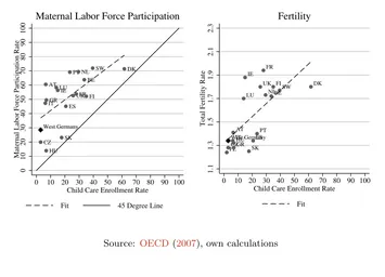
Figure 1 shows for a cross-section of EU countries (those which are also in the OECD) the
signif-icant positive correlation of the fraction of children aged zero to two enrolled in a paid child care arrangement, e.g. in form of a daycare center or a nanny, with the labor force participation rate of
mothers with children aged zero to two and the total fertility rate.1 Clearly, these correlations do
not necessarily reflect causality and (due to data availability) only display the actual enrollment rates and not the provision rates of child care. Hence, with regard to the main question asked in this paper these figures do not permit to draw conclusions on how far (not) providing child care constitutes a barrier or disincentive for female labor force participation and fertility choices. Moreover, the relationships crucially hinge on the age of the children. For children aged three to five the previously significant positive correlations become negative or much weaker and are no
longer statistically significant, see Figure 2. This suggests a very different role of child care for
maternal labor force participation decisions in the two age groups. In this context, Figures1 and2
reveal another important relationship. The labor force participation rate of mothers with children aged zero to two exceeds the corresponding child care enrollment rate on average by 29 percentage points. To the contrary, for mothers with children aged three to five the child care enrollment rate exceeds the maternal labor force participation rate on average by 19 percentage points. Put differently, paid child care is used heavily by non-working mothers (of children between age three and five) whereas a substantial fraction of mothers (of children below age three) works without using any paid child care. This gap cannot be explained by the usage of nannies or alike as those arrangements are already included in paid child care enrollment. Note that this also holds in the
1
Figure 1: Child Care Enrollment of Children Aged 0 to 2 in the EU CZ IT AT HU GR LUIE SK ES PT UKFR NL BE FI SW DK West Germany 0 10 20 30 40 50 60 70 80 90 100
Maternal Labor Force Participation Rate
0 10 20 30 40 50 60 70 80 90 100
Child Care Enrollment Rate
Fit 45 Degree Line
Maternal Labor Force Participation
PLCZ IT AT HU GR LU IE SK ES PT UK FR NLBE FI SW DK West Germany 1.1 1.3 1.5 1.7 1.9 2.1 2.3
Total Fertility Rate
0 10 20 30 40 50 60 70 80 90 100
Child Care Enrollment Rate
Fit
Fertility
Source: OECD(2007), own calculations
Figure 2: Child Care Enrollment of Children Aged 3 to 5 in the EU
FI GR NL LU SK AT PT UK CZ SW HU DK ES BE IT FR West Germany 0 10 20 30 40 50 60 70 80 90 100
Maternal Labor Force Participation Rate
0 10 20 30 40 50 60 70 80 90 100
Child Care Enrollment Rate
Fit 45 Degree Line
Maternal Labor Force Participation
PL FI GR IE NL LU SK ATPT UK CZ SW HU DK ES BE IT FR West Germany 1.1 1.3 1.5 1.7 1.9 2.1 2.3
Total Fertility Rate
0 10 20 30 40 50 60 70 80 90 100
Child Care Enrollment Rate
Fit
Fertility
[image:4.595.125.485.495.746.2]US and Canada: 18.5 and 39.7 percentage points, respectively, more of the mothers with children
aged zero to two are working than using paid child care, seeOECD (2007).
The observation that unpaid child care is a common choice has already been acknowledged in one of
the earliest economic studies of child care byHeckman(1974) but has been ignored in many recent
analyses. Blau and Currie(2006) summarize the results for a wide range of studies for the US (Table
5 in there) which employ static discrete choice models to investigate the interaction between child
care and maternal labor force participation. Among those only three,Ribar(1995),Blau and Hagy
(1998), andTekin(2007) include non-paid, non-maternal child care as choice. However,Blau(2003)
shows that the assumption that paid care is always the relevant non-maternal child care option leads to inconsistent parameter estimates which as a consequence impacts the result of any counterfactual policy analysis. Recent dynamic models on female labor supply with a focus on paid child care,
e.g. Attanasio, Low, and Sanchez-Marcos (2008), Domeij and Klein (2010), Fehr and Ujhelyiova
(2010), and Haan and Wrohlich (2011), are as well prone to this critique as all assume that each
hour of maternal work requires one hour of paid child care.
The first contribution of this paper is to introduce non-paid, non-maternal child care into a dynamic setting which features returns to experience. Second, by distinguishing paid child care between publicly (subsidized) and market (non-subsidized) provided arrangements the setup allows me to address the policy question asked at the beginning, namely in how far governments can influence maternal labor force participation by increasing the provision of child care. Finally, this question
is extended to fertility by making it as well a choice variable.2
The analysis is undertaken with a quantitative, dynamic life-cycle model which is calibrated to a
sample of West German married females.3 West Germany constitutes an ideal candidate for the
following reasons. First, in terms of data availability, the German Socioeconomic Panel (GSOEP) is the only European household panel with continuous information on paid child care usage along the extensive and intensive (part- vs. full-time) margin. Moreover, the characteristics of the German child care market permit to infer from the GSOEP whether a child attends publicly (subsidized) or market (non-subsidized) provided child care. In addition, the number of subsidized child care slots per hundred children is available from the German Statistical Office. Second, the low maternal labor force participation, child care enrollment and fertility rates in Germany are representative for Continental Europe (with the exception of France and BeNeLux), such that the results from counterfactual policy experiments should be of interest to other Continental European countries.
The paper contributes to the literature that uses dynamic life-cycle models to evaluate family
poli-cies, as e.g. in Guner and Knowles(2009) and Erosa, Fuster, and Restuccia (2010), by evaluating
2
Fehr and Ujhelyiova(2010), andHaan and Wrohlich(2011) also endogenize fertility but, as already noted, ignore the option of non-paid, non-maternal child care. Del Boca (2002), and Del Boca and Sauer (2009) constitute a special case. They investigate the impact of child care provision as an “economy-wide factor” on fertility and maternal labor force participation without modeling child care as a choice or as a requirement for working mothers.
Blau and Robins(1989),Blau and Robins(1991) for the US,Kravdal (1996) for Norway andHank and Kreyenfeld
(2003) for Germany conduct a reduced form analysis of the role of child care for fertility and partly maternal labor force participation. Lehrer and Kawasaki(1985) andMason and Kuhlthau(1992) investigate in how fare child care affects birth intensions.
3
a reform that aims at implementing the target for the provision of child care for children aged zero to two set by the European Council at the 2002 Barcelona meeting. Under this reform all working females are granted access to subsidized child care. Such a reform has been implemented in Germany in October 2010. According to my results the lack of subsidized child care constitutes indeed for some females a barrier to participate in the labor market and depresses fertility. The predicted increase of the labor force participation rate is 23% (7.4 percentage points) for moth-ers with children aged zero to two. This response is very close to the empirically estimates by
Baker, Gruber, and Milligan (2008) and Lefebvre and Merrigan (2008) for the late 1990s in
Que-bec after the introduction of a similar policy. Moreover, the implied price elasticity of maternal labor force participation with respect to paid child care is exactly in the range of estimates listed
inBlau and Currie(2006) for the models that feature as well a non-paid, non-maternal child care
choice, whereas models that require each hour of maternal labor supply to be backed by one hour of paid child care are associated with much higher price elasticities (in absolute terms). The child care enrollment rate under the new policy is 41% and thus “overshoots” the targeted level of 33% while the effect on fertility is only modest, plus 3% or 0.05 children per female. Despite this small reaction, it is important to endogenize fertility as the aggregate effects on female labor supply are otherwise significantly overestimated and as a consequence the costs of the reform underestimated.
I consider a further reform which is a natural extension of the previous reform and grants access to subsidized part-time child care for all children aged zero to two, i.e. unconditional on the maternal labor force status. This reform results in a higher child care enrollment rate but has neither an impact on maternal labor force participation nor on fertility relative to the first reform. Hence, only females that are constrained in their labor force participation choice by the lack of subsidized child care are also constrained in their fertility choice.
The structure of the paper is as follows: In Section 2, I describe the data set, and how the sample
is selected and constructed. Section 3 documents facts about maternal labor force participation,
child care usage and the supply of subsidized child care in West Germany. I introduce the model
in Section 4, discuss the calibration in Section5 and the model evaluation in Section 6. Section 7
presents the results from a set of counterfactual policy experiments and Section8 concludes.
2
Data
The analysis in this paper is based on the German Socioeconomic Panel (GSOEP), an annual
household panel comparable in scope to the American PSID.4The GSOEP provides all information
required for the pursued question, i.e. female cohabitation, labor force participation and birth histories, child care enrollment choices, paid child care fees, and income. In particular, it is the only European household panel with information on paid child care usage along the extensive and
intensive (part- vs. full-time) margin over the entire sample period.5 The data are drawn from the
first wave in 1984 through 2007 spanning the years 1983 to 2006 since the variables on labor force participation and income refer to the year prior to each interview.
4
A detailed description of the GSOEP can be found inWagner, Frick, and Schupp(2007).
5
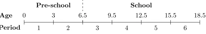
Figure 3: A Child’s Life from Birth to Adulthood
Pre-school School Age
Period
0 3 6.5 9.5 12.5 15.5 18.5
1 2 3 4 5 6
Following the common practice in the literature on female labor supply and fertility, only females living in a continuous relationship (marriage or cohabitation) with the same partner are included
in the sample.6 I include only the most recent relationship but require that it is still intact at the
last interview and that all children (if present) are from the current partner. The analysis focuses entirely on West German females and consequently only females that lived there throughout the whole observation period are considered. Finally, given a trade-off between sample size and poten-tial cohort effects females born between 1955 and 1975 are included. The number of individuals
satisfying the respective selection criteria are shown in TableA.1 in AppendixA.1.
Maternal labor force participation and child care enrollment choices by the children’s age constitute
the core of the analysis in this paper. Similarly to Apps and Rees(2005), my focus is however not
on the maternal labor force participation status in each month of a child’s life but during the different stages of a child’s adolescence. For pre-school ages I follow the usual convention and split them up in two periods, ages zero to two and ages three to mandatory school age where children in Germany are on average six and a half years old. To keep the periods at a similar length,
the subsequent age brackets cover three years until adulthood is reached. Figure 3 summarizes
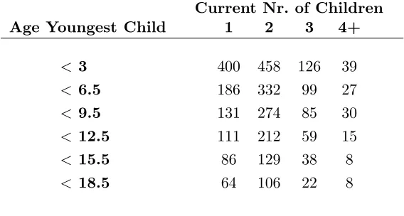
this mapping. Table 1 presents the final number of observations for each period grouped by the
current number of children, e.g. the sample contains 458 females with currently two children and the youngest child being younger than three. Given the low number of observations for females with currently four and more children, the analysis on maternal labor force participation and child care enrollment in this paper focuses on females with one to three children only.
For each period the female labor supply is constructed similar to Francesconi(2002): I assign 0 to
each month in which the female does not work, 0.5 to each month in which she works part-time and
1 to each month in which she works full-time.7 The period labor force participation status is then
defined by the mean over all months. Period means below 0.25 correspond to not working, between 0.25 and 0.75 to part-time working, and above 0.75 to full-time working. As an implication, a female working part-time in each month of a period and one not working in the first half of a period but full-time in the second half have the same period labor force participation status, namely part-time working. In line with the objective of this paper this definition reflects how much a female has worked in total during certain stages of her children’s adolescence.
6
The implied selection bias of focussing on this group of females may go in opposite directions. For example, the unobservables that produce long-term relationships could make women more desirable in the labor market (e.g., good communication and conflict management skills) but could also reflect preferences for non-market activities as household production. A more detailed discussion can be found inFrancesconi(2002).
7
Table 1: Observations
Current Nr. of Children Age Youngest Child 1 2 3 4+
< 3 400 458 126 39
< 6.5 186 332 99 27
< 9.5 131 274 85 30
< 12.5 111 212 59 15
< 15.5 86 129 38 8
< 18.5 64 106 22 8
Note: To avoid biased means if there are trends in labor partici-pation or child care enrollment within a period, i.e. during a stage of a child’s adolescence, only periods that are neither interrupted by another birth nor left or right censored through the first or last interview are included.
The GSOEP asks for enrollment in paid child care, distinguishing between two different categories, namely daycare centers and nannies, and whether the child is enrolled part- (during the morning or afternoon) or full-time (all day). Since virtually all daycare centers receive public subsidies I use this category for publicly provided child care, henceforth called subsidized child care. During the observation period parents could claim only in special circumstances, e.g. severe diseases, financial support for hiring a nanny reflecting that nannies rather constitute a market arrangement. Ac-cordingly, I label them as non-subsidized child care. The corresponding period enrollment status for subsidized and non-subsidized child care is then calculated in the same way as the labor force
participation status.8 Finally, aggregate statistics on the provision of subsidized part- and full-time
child care by age groups (zero to two and three to six and a half) are available from the Germans
Statistical Office.9
3
Stylized Facts
This section documents labor force participation and child care enrollment choices for the selected
sample of West German married females.10 These facts will be either used as calibration targets
for the model developed in Section 4 or for the evaluation of the model fit. I further describe
8
The child care enrollment status is only known for the interview month. In AppendixA.2I discuss the imputation for the remaining months and outline how I deal with changes in the GSOEP child care questions over time.
9
In AppendixA.3I describe how I calculate the period provision rates of subsidized child care such that they are consistent with the definition of the period labor force participation and child care enrollment status as discussed before.
10
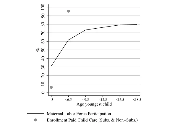
Figure 4: Maternal Labor Force Participation and Child Care
0
10
20
30
40
50
60
70
80
90
100
%
<3 <6.5 <9.5 <12.5 <15.5 <18.5
Age youngest child
Maternal Labor Force Participation
Enrollment Paid Child Care (Subs. & Non−Subs.)
features of the German child care market, namely the provision of subsidized child care as well as the parental fees for subsidized and non-subsidized child care, that can be considered as exogenous for the individual choices and will serve as model inputs.
I start with the discussion of the total maternal labor force participation and child care enrollment rates and will turn to the part- and full-time differences further below.
3.1 Maternal Labor Force Participation and Child Care
Figure4 shows that the maternal labor force participation rate increases with the youngest child’s
age but at a strongly decreasing rate. In particular, the major increase happens during pre-school ages (from 31% to 61%) and at school entry (from 61% to 73%). The subsequent increases are far smaller and when the youngest child turns adult (ages 16 to 18.5) 80% of the mothers in the sample are working. The increase of the child care enrollment rate, comprising subsidized and non-subsidized child care, from 6% for children aged zero to two to 95% for children aged three to six and a half is much larger than the corresponding increase in the maternal labor force participation rate. Accordingly, the selected sample displays a similar relationship as the cross-section of EU
countries shown in Figures 1 and 2: the maternal labor force participation rate for the age group
zero to two is much larger than the enrollment rate in paid child care (31% vs. 6%), whereas the opposite is true for the age group three to six and a half (61% vs. 95%).
Table2takes a closer look at this relationship. Only 13.7% of the working mothers whose youngest
Table 2: Child Care Enrollment Conditional on Maternal Labor Force Participation Status
Ages 0 to 2 Ages 3 to 6.5
At least part-time care
Not Working 2.9 93.2
[image:10.595.105.509.306.402.2]Working 13.7 96.7
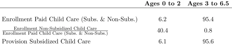
Table 3: Child Care Enrollment and Provision
Ages 0 to 2 Ages 3 to 6.5
Enrollment Paid Child Care (Subs. & Non-Subs.) 6.2 95.4
Enrollment Non-Subsidized Child Care
Enrollment Paid Child Care (Subs. & Non-Subs.) 40.4 0.8
Provision Subsidized Child Care 6.1 95.6
family members or friends might also take care of the children at no monetary costs. Since the total enrollment rate in paid child care is 95% for children aged three to six and a half, it is not surprising that the respective conditional child care enrollment rates hardly vary with the maternal labor force participation status. Overall, the correlation between the maternal labor force participation and child care enrollment rate is weak whereas the correlation of both variables, particularly the child care enrollment rate, with the children’s age is large.
Table 3 shows that non-subsidized child care is an important source of paid child care in relative
terms for children aged zero to two: among the children in this age group enrolled in paid child care, 40.4% are enrolled in non-subsidized child care, either exclusively or in addition to subsidized child care. However, in absolute terms this is still negligible (amounting to 2.5% of all children aged zero to two). For children aged three to six and half non-subsidized child care is hardly used independent of whether measured in relative or in absolute terms. This latter result is not surprising as the fees for non-subsidized child care are three to four times as expensive as subsidized child care (see Table
C.6in Appendix C.3) and, as shown in the third row of Table 3, subsidized child care is available
for nearly all children in that age group. In contrast, only for 6.1% of the children aged zero to two a subsidized child care slot is available.
The huge disparity of the provision rates between the two age groups stems from the historical objective to subsidize child care in Germany, namely to offer affordable, high quality pre-school
education for children from age three onwards, seeKreyenfeld, Spieß, and Wagner(2002). Wrohlich
(2008) documents a substantial excess demand for subsidized child care for children aged zero to
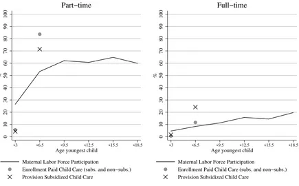
Figure 5: Maternal Labor Force Participation and Child Care: Part- vs. Full-time
0
10
20
30
40
50
60
70
80
90
100
%
<3 <6.5 <9.5 <12.5 <15.5 <18.5
Age youngest child
Maternal Labor Force Participation
Enrollment Paid Child Care (subs. and non−subs.) Provision Subsidized Child Care
Part−time
0
10
20
30
40
50
60
70
80
90
100
%
<3 <6.5 <9.5 <12.5 <15.5 <18.5
Age youngest child
Maternal Labor Force Participation
Enrollment Paid Child Care (subs. and non−subs.) Provision Subsidized Child Care
Full−time
zero to two the provision rate exceeds the actual enrollment in subsidized child care (given that a substantial fraction is enrolled in non-subsidized child care) should therefore rather be interpreted as a mismatch of supply and demand of subsidized slots than as an excess supply.
3.2 Part- vs. Full-time
Another important feature of the data is the prevalence of part-time maternal labor force participa-tion, part-time enrollment in paid child care (again, subsidized and non-subsidized) and provision
of part-time subsidized child care, see Figure5. The profile of the total maternal labor force
partici-pation rate follows the profile of the part-time maternal labor force participartici-pation rate until age nine and a half, while the increase afterwards mainly stems from the full-time labor force participation rate. Although the full-time child care enrollment for children aged three to six and a half is above the corresponding full-time maternal labor force participation rate, the usage of non-paid child care is still pervasive among full-time working mothers in this age group. Only 32.4% of them actually use full-time child care. About three fourth of the subsidized child care slots are part-time with the actual enrollment rates in part-time child care being even higher because some full-time slots
are only used part-time.11
11
3.3 Summary Key Facts
The facts documented in this section about labor force participation of married females with chil-dren and their child care enrollment decisions can be summarized as follows:
1. The maternal labor force participation rate grows as the children age but at a strongly decreasing rate.
2. Many non-working females use paid child care and many working females do not use paid child care.
3. Non-subsidized child care is only important for children aged zero to two but only in relative terms.
4. While subsidized child care is three to four times as cheap as non-subsidized child care, it is only provided for very few children aged zero to two. Although for nearly all children aged three to six and a half a subsidized child care slot is available, the majority of those slots is only part-time.
5. For both, child care enrollment and maternal labor force participation, the part-time rates exceed the full-time rates.
In the next section, I develop a life-cycle model to explain the set of presented facts on maternal labor force participation and child care enrollment taken as given the supply of subsidized child care slots and parental fees for subsidized and non-subsidized child care.
4
The Model
This section introduces a stylized life-cycle model for married females featuring fertility, labor force participation and child care choices.
4.1 Demographics
A female lives for six periods, each of three year length, reflecting the distinctive stages of a child’s
adolescence, as shown in Figure 3.12 At the beginning of her life she is exogenously matched with
a man and then chooses how many children to have. Both the husband and the children stay with her throughout her whole life. If a female chooses to have more than one child, all children are born as multiples. This simplifying assumption is made for tractability.
driven by mothers working very few hours. Conditional on working, only 15.6% (10.6%) of those whose youngest child is of age zero to two (three to six and a half) are working less than 10 hours. The detailed results are available upon request.
12
4.2 Endowments
Females and their husbands are indexed by income shocksǫandǫ∗ which determine the stochastic
component of their market incomes. Asterisks refer to parameters for the husband. Both spouses
are assigned initial income shocks (ǫ1, ǫ∗1) in period one which subsequently evolve stochastically
over time according to an AR(1) process:
ǫt=ρǫt−1+εt with εt∼N(0, σε2) ǫ∗t =ρ∗ǫ∗t−1+ε∗t withε∗t ∼N(0, σ2ε∗)
(1)
In the first two periods while children are not yet in school, females can enroll them in subsidized and/or non-subsidized child care. Both types of child care are perfect substitutes with the exception
of the price and availability. In contrast to non-subsidized child care, I assume as inWrohlich(2006)
and Haan and Wrohlich(2011) that access to subsidized child care slots, denoted asat, is rationed
and randomly assigned to mothers by a lottery with age-dependent success probabilities. These success probabilities are assumed to be independent of the maternal labor force participation status or number of children as their is no information in the data that would allow me to identify such dependencies.
4.3 Preferences
The female is assumed to be the household’s sole decision maker, i.e. she has the full bargaining
power. A childless woman (n= 0) receives utility from her share of household consumption (ψ(n)ct)
and leisure which is the time endowment of one less time worked in the market lt:
ut,n=0 =
(ψ(n)ct)1−γ
0 −1
1−γ0
+δ1
(1−lt)1−γ1 −1
1−γ1
. (2)
Household consumption (ct) is transformed into the consumption realized by an adult, the female’s
share, using the OECD equivalence scale:
ψ(n) = 1
1.7 + 0.5n. (3)
The utility function for a mother (n >0) is different. Her leisure is further reduced by the time
caring for her children (mt) while she receives in addition utility from having children (N) and
child quality (Qt):
ut,n>0 =
(ψ(n)ct)1−γ0−1
1−γ0
+δ1(1−lt−mt)
1−γ1−1
1−γ1
+δ2N+δ3Qt, (4)
whereδi∀i= 1,2,3 measure the contribution of each part to total utility relative to the utility from
consumption. This general specification is relatively standard, see e.g.Greenwood, Guner, and Knowles
ad-ditional parts. The utility from havingn >0 children is
N= (1 +n)
1−γ2 −1
1−γ2
−ζ. (5)
The first component reflects a decreasing marginal utility in the number of children while the second
component (ζ) is a rescaling factor that only affects then= 0 vs. n= 1 choice but not any other
decision conditional on having children. It counteracts the large utility gain females receive from having the first child induced by the first component. Anticipating the calibration results such a
fixed cost of having children, i.e. ζ > 0, is quantitatively needed to induce some females to not
have children. Setting ζ = 0 this result could be also achieved with a sufficiently low value of the
utility weight δ2. In this case however the empirically observed fertility distribution in terms of
number of children could not be matched any longer because the utility differences from having another child would be too small. A further alternative is a model with a fixed time cost of having
children instead of the rescaling factorζ. The calibrated fixed cost needed to match the fraction of
females without children would however have to be that large that essentially no mother would be
willing to work full-time any longer. 13 To sum up, introducing a fixed cost of having children in
this fashion is a pragmatic way to generate the observed fertility distribution (in terms of number of children) without affecting other margins drastically.
The child quality termQtintroduces the main behavioral trade-offs. The concrete specification is
motivated by the facts outlined in Section3and similar toRibar(1995). As their mothers, children
have a time constraint:
mt+ccs,t+ccns,t+ccnp,t= 1. (6)
They either spend time with their mother (mt), are taken care of in a paid child care arrangement,
either subsidized (ccs,t) or non-subsidized (ccs,t), or in a non-paid child care arrangement (ccnp,t).
These inputs affect child quality Qt in the following way:
Qt=ξ(t)mγ
3
t −φ(t)cc φ2
np,t =ξ(t)m γ3
t −φ(t) (1−mt−ccs,t−ccns,t)φ
2
. (7)
Note that both types of paid child care, i.e. subsidized and non-subsidized, are perfect substitutes
with the exception of the price and availability. As inRibar (1995), the effect of paid child care to
overall child quality is ambiguous and depends only on the quality of paid care relative to maternal and non-paid care. Specifically, I assume that child quality is increasing in maternal time spend
with the children mt and decreasing in the usage of non-paid child care.14 This latter mechanism
is needed to explain usage of paid child care (which reduces resources for consumption) while
non-paid child care is available, see also Blau and Hagy (1998), Wrohlich (2006) and Tekin (2007).15
Thus, the above setup does not require that for each unit of labor supply one unit of paid child
13
Using a very similar model with such time costs, Greenwood, Guner, and Knowles (2003) also do not predict any childless females because their time costs are still to low.
14
Ribar(1995) specifies his estimated model the other way around than Equation (7), i.e. he includes paid child care usage instead of non-paid child care usage in the utility function. Since the three modes of care, paid, non-paid and maternal are linked through the time constraint (6) this should not affect the results.
15
care has to be bought since instead non-paid child care could be used. Without this assumption
the documented fact that not all working females use paid child care, compare Table 2, could not
be generated. Possible interpretations for the utility costs of paid child care could be that non-paid child care arrangements provide lower quality child care than non-paid child care arrangements or mothers, the effort to organize care provided by grandparents, other family members or friends, the foregone joint leisure-time with the husband if he takes care of the children or the disutility of taking care of the children while working from home (e.g. as self-employed). Still there is no reason to believe that families actually have direct negative preferences regarding unpaid care, but
the approach is a flexible way to proxy for the direct costs of non-paid care, seeRibar(1995). This
discussion also reveals that it would be too far stretched to interpretQtas children’s human capital
which is also not doneRibar(1995),Blau and Hagy(1998),Wrohlich(2006) andTekin(2007). For
a recent structural approach to estimate the effect of employment and child care decisions of married
mothers on children’s cognitive development, see e.g. Bernal (2008).
Hotz and Miller (1988) assume that mothers incur a time cost of having children that declines
geometrically with the age of the children to capture that children of different ages have different needs. I make a similar assumption and allow for the possibility that the utility mothers receive from spending time with their children declines geometrically over time, i.e. as the children get older. This increases both the incentive to use (more) paid and non-paid child care and to participate (more) in the labor market as the children get older. The speed of the reduction is given by the
parameter ξ1 >0 whereas the lower bound, i.e. the utility in the last period when children are of
age 15.5 to 18.5, is governed by ξ2∈[0,1] through the following linear transformation:
ξ(t) =ξ2+
t−ξ1−T−ξ1
1−T−ξ1 (1−ξ2) for t= 1, . . . , T and T = 6. (8)
With the focus being on pre-school child care, I assume that the costs of non-paid child care usage only accrue while children are of pre-school age, i.e.
φ(t) =
φ1 fort≤2
0 else. (9)
Put differently, a mother does not have to organize child care if she does not spend time with her
children after the end of the school day. As inRibar(1995),Blau and Hagy(1998),Wrohlich(2006)
andTekin(2007), I assume that every female can use as much non-paid child care as she desires. A
possible justification for this assumption is that the husbands could always take care of the children while the female is working. The only requirement, given that all husbands are working full-time, is that the spouses are working at different times of the day. At least in principle this arrangement is open to all females, although frictions in the real world labor market might limit the choice
of when to work. Table B.1 in AppendixB presents further evidence in favor of the assumption
of unconstrained access to non-paid child care. The children’s grandparents, i.e. the female’s or husband’s parents, are (next to the husband) the most likely provider of non-paid child care. The geographical distance towards grandparents is probably one of the most important sources for
heterogeneity in access to non-paid child care. TableB.1shows that this heterogeneity does hardly
child care, it is clearly not a rejection of the assumption.
4.4 Budget Constraint
The per-period budget constraint is given by:
ct=τ[yt(lt, xt, ǫt), yt∗(t, ǫ∗t)]−fcc[n, t, ccs,t, ccns,t, yt, yt∗] + Υ [n, t, lt]. (10)
The function τ calculates the after tax household income from the female’s (yt) and husband’s
(yt∗) gross income. The latter depends on two components: a deterministic component in time t,
i.e. all husbands are assumed to work full-time and thus accumulate full-time experience,16 and a
stochastic component represented by the husband’s current period income shock (ǫ∗t). In contrast,
the female’s income depends on her labor supply (lt), accumulated experience (xt) through past
labor force participation
xt=xt−1+lt−1, with x1 = 0 (11)
and her current period income shock (ǫt). Similar to the vast majority of structural models
in-vestigating labor supply and fertility choices of married females, see e.g. Hotz and Miller (1988),
Francesconi (2002) or Haan and Wrohlich (2011), I abstract from savings. Child care fees fcc
de-pend on the number (n) and age (t) of the children, the utilized amount of subsidized (ccs,t) and
non-subsidized (ccns,t) child care as well as the gross household income. In addition, households
receive transfers Υ conditional on the time period/age of the children (t) and choices (n, lt). The
functional forms for the gross incomes y and y∗, the tax schedule τ, the child care fees fcc and
transfers Υ are specified further below in Section5.1.
4.5 Choice Variables
All choices are assumed to be discrete. Labor supplylt can take on three values:
lt=
0 for non-working
1
4 for part-time work
1
2 for full-time work
∀ t= 1, . . . ,6. (12)
If the (non-sleeping) time endowment would be 16 hours, then part-time labor force participation
would correspond to four and full-time work to eight hours. Similarly, subsidized ccs,t and
non-subsidized child careccns,t can take on three values:
cci,t =
0 for no paid child care
1
4 for paid part-time child care
1
2 for paid full-time child care
∀t= 1,2 and i=s, ns. (13)
The actual choice of subsidized child care is however restricted by the access at to a subsidized
child care slot:
ccs,t≤at ∀t= 1,2, (14)
16
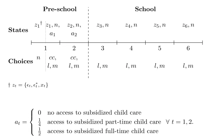
Figure 6: Life Cycle
States
Choices
†zt={ǫt, ǫ∗
t, xt}
Pre-school School
1
z1†
n z1, n,
a1
l, m cc,
2
z2, n,
a2
l, m cc,
3
z3, n
l, m
4
z4, n
l, m
5
z5, n
l, m
6
z6, n
l, m
with
at=
0 no access to subsidized child care
1
4 access to subsidized part-time child care
1
2 access to subsidized full-time child care
∀ t= 1,2. (15)
As already mentioned, the access to a subsidized child care slot is determined by a lottery with age- and type-dependent, i.e. part- or full-time, success probabilities. Paid child care in subsidized and non-subsidized arrangements is restricted to
ccs,t+ccns,t ≤
1
2 ∀ t= 1,2, (16)
i.e. child care facilities are only open during the first half of the day in the morning and early afternoon. A mother can still spend time with her children in the late afternoon and evening such that in principle
mt∈
0,1
4,
1
2,
3
4,1
. (17)
However, while she is working and/or the children are in paid child care or later in life in mandatory
costless schooling (st), she cannot spend any time with her children:
mt≤
1−max{lt, ccs,t+ccns,t} ∀ t≤2
1−max{lt, st} ∀3≤t≤6. (18)
4.6 Dynamic Problem
Figure 6 presents the timing of events during a female’s life which is defined by the stages of her
children’s adolescence (compare also Figure 3). The term zt combines the income shocks of both
spouses (ǫt, ǫ∗t) and the female’s experience level (xt, with x1 = 0). The first period is split up in
two stages with different state and decision variables. In the first stage, the initial income shocks
uncertainty with respect to the access to subsidized child care:
max
n {Ea1V(1, ǫ1, ǫ
∗
1, x1, n, a1), n= 0,1,2, ..., N}, (19)
with V(·) being the female’s value function. Once the optimal number of children (n) is chosen,
n becomes a state variable as the children stay with the mother throughout her entire life. After
access to subsidized child care is determined by the lottery, the female decides on her labor supply
(l1) and those with children, on how much time to spend with them (m1) and on their enrollment
in subsidized child care (ccs,1), possibly restricted by a1, and non-subsidized child care (ccns,1).
The following Bellman equation represents the female’s problem in the second stage:
V(1, ǫ1, ǫ∗1, x1, n, a1) = max
m,l,ccs,ccns
u1+βEǫ,ǫ∗,a2V(2, ǫ2, ǫ∗2, x2, n, a2)
subject to (10), (11), (14), (16) and (18).
(20)
u1is the period-specific utility function (Equation (4)) andβis the discount factor. At the beginning
of period two, the new income shocks (ǫt, ǫ∗t) realize according to the AR(1) process specified in
Equation (1) and access to child care (a2) is drawn from a new lottery. The set of choice variables
in period two is identical to the second decision stage in period one and the value function is given by
V(2, ǫ2, ǫ∗2, x2, n, a2) = max
m,l,ccs,ccns
u2+βEǫ,ǫ∗V(3, ǫ3, ǫ∗3, x3, n,0)
subject to (10), (11), (14), (16) and (18).
(21)
From period three onwards, children attend mandatory school and females cannot use child care
anymore (at = 0 for t ≥ 3). Hence, a female only decides on how much to work and how much
time to spend with her children:
V(t, ǫt, ǫ∗t, xt, n,0) =max
m,l ut+βEǫ,ǫ
∗V(t+ 1, ǫt+1, ǫ∗t
+1, xt+1, n,0) ∀ 3≤t≤6
subject to (10), (11) and (18)
and V(7, . . .) = 0.
(22)
4.7 Maternal Leave
An important element affecting labor force participation decisions of females with children aged zero to two is the German maternal leave regulation. It permits every mother who worked until the birth of a child to return to her pre-birth employer at her pre-birth wage within three years after birth. Since in the model life starts with the birth decision, there is no pre-birth labor supply
and I therefore grant all females the right to go on maternal leave.17 Relevant in this setup is
the stochastic part of income. By construction, part- and full-time working mothers work at their initial or pre-birth wage income shock in period one. Hence, the maternal leave regulation has only
to be modeled explicitly for mothers that do not work in the first period, i.e. for which l1 = 0 or
equivalently x2 = 0. I assume that they draw a new income shock at the beginning of the second
17
period according to Equation (1) (e.g. an offer for a new position) but can opt for the pre-birth income shock (e.g. return to the pre-birth position) such that the offered wage in the second period
is given by y2(l2, x2= 0,max{ǫ1, ǫ2}). The third period income shock is then determined by
ǫ3 =
ρ max{ǫ1, ǫ2}+ε3 if l1 = 0, l2 >0
ρǫ2+ε3 else.
5
Calibration
In the following paragraphs, I specify the functional forms for the exogenous model inputs which are, where applicable, either presented as monthly or annual values. When used in the model all variables are transformed to correspond to the model period length of three years. All monetary
values are expressed in real terms in 2008e. In this section I further discuss the target moments
for the calibration exercise and the calibrated preference parameters.
5.1 Functional Forms
5.1.1 Income
Husbands In line with the data, all husbands are assumed to work full-time and thus accumulate
full-time experience. I assume that the log of their gross income y∗t is a concave function of
experience and hence of time in the model or, respectively, of the youngest child’s age in the data:
lny∗t =η0∗+η1∗(t−1) +η∗2(t−1)2+ǫ∗t (23)
The gross full-time income yt(lt, xt, ǫt) of a female is given by a classical Mincer (1974) earnings
equation with returns to experience, where full-time work lt= 12, see Equation (12). As a
normal-izationxtis multiplied by two (˜xt= 2xt) such that part-time work increases ˜xby 0.5 and full-time
work by 1:
lnyt=η0+η1xt˜ +η2x˜2t +ǫt. (24)
I assume that there is no part-time penalty, i.e. the gross part-time income is half of the gross full-time income for the same level of experience and the same income shock.
Appendix C.1 describes how the income processes are estimated. Given the specific structure of
the model, standard estimates from the literature cannot be used. Moreover the feature of joint income taxation (see below) requires to to estimate a gross income process and apply the tax code afterwards, instead of estimating a net income directly, in order to capture the appropriate
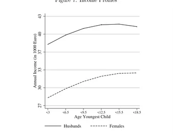
incentives for married females to work. The predicted income profiles are displayed in Figure 7.
For the numerical solution of the model, the AR(1) process for the income shock (Equation (1)) is
Figure 7: Income Profiles
27
30
33
37
40
43
Annual Income (in 1000 Euro)
<3 <6.5 <9.5 <12.5 <15.5 <18.5
Age Youngest Child Husbands Females
5.1.2 Taxes and Transfers
The tax code implemented in the model incorporates the three key elements of the German tax system: mandatory social security contributions, progressive and joint taxation.
Employees, excluding civil servants, have to make mandatory contributions to the pension system, unemployment, long-term care and public health insurance which accrue proportionally to income up to a contribution limit. In the model I use the average contribution limits and rates for each type of insurance over the years 1983 to 2006. Similarly, the implemented tax code is based on the average income taxes over the sample period. The construction of the tax code is described
in AppendixC.2which also shows the final social security contributions and tax rates used in the
model. In Germany legally married couples are taxed jointly, i.e. the tax code is applied to half of the sum of the spouses’ incomes and the resulting tax burden is doubled. By the progressivity of the tax system the joint net income is always at least as large as the sum of the individually taxed incomes. Although my sample includes some cohabitating but not legally married couples, I apply joint taxation.
The transfers considered include the average child benefits over the the years 1983 through 2006 which are paid each period depending on the total number of children. The average benefit per
child is slightly increasing in the number children, see Table C.4 in Appendix C.2. Based on
the description in Ludsteck and Schoenberg(2007) non- and part-time working mothers receive in
period one a maternity benefit of 2414.19 e which comprises the maternity benefits paid during
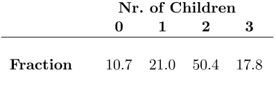
Table 4: Fertility Distribution
Nr. of Children
0 1 2 3
Fraction 10.7 21.0 50.4 17.8
Note: Figures are based on the 1140 females from the sample selected in Section2who have completed their fertile period, assumed to end at the age of forty.
5.1.3 Child Care Fees
The child care fees fcc[n, t, ccs,t, ccns,t, yt, y∗t] consist of two parts: the per-child fees for subsidized
and non-subsidized child care multiplied by the number of children. The per-child fees for subsidized
child care are the predicted values from a Tobit-regression with censoring at 0eand at 447.72 e,
the lowest and highest observed monthly fee for subsidized child care with the following set of regressors: an intercept, a full-time dummy, a dummy for ages zero to two, number of further
siblings enrolled in subsidized child care, and household income.18 The per-child fees for
non-subsidized child care are the predicted values from an OLS-regression on a constant and a full-time dummy, the only two regressors that turned out to be statistically significant. The coefficients for
both regressions and predicted fees are shown in TablesC.5and C.6in AppendixC.3.
5.1.4 Subsidized Child Care Provision Rates
The age- and type-dependent, i.e. part- and full-time, success probabilities in the lottery
deter-mining access to subsidized child care are taken from Figure5 and are also shown in Table A.3in
AppendixA.3.
5.1.5 School Hours
I assume that children attend school part-time (st = 14) in periods three and four, i.e. for ages
seven to 12.5, and full-time (st= 12) in periods five and six, i.e. for ages 13 to 18.5. Schooling hours
matter by limiting the maximum amount of time the mother can spend with her children, compare
Equation (18).
18
5.2 Data Targets
The discount factor β is set to 1.1043 as in Kydland and Prescott (1982). The remaining 12
preference parameters are calibrated by matching 12 moments that are grouped in three data categories. I assign each parameter to the group where the influence is felt the heaviest and try to argue as far as possible in how far the data are informative about the respective parameter values. Since however aggregate statistics are matched, as opposed to individual data, and all parameters jointly determine the model statistics, the following discussion is only suggestive and informal.
Fertility While ζ reflects the fixed costs of having a positive number of children, δ2 and γ2 gov-ern the direct utility of having children. Accordingly these three preference parameters strongly influence the fertility outcomes. I target the fraction of females without, with one and with two
children. Table 4 shows the empirical fertility distribution for a maximum of three children per
female which are adjusted for the fact that around 3.5% of all couples are unable to get children
at all, see Robert Koch Institut and German Statistical Office(2004).
Labor Force Participation Since the focus of the analysis is on child care and thus the pre-school ages, I target the average (over all mothers) part- and full-time labor force participation rate when children are of ages zero to two and three to six and a half. In addition, both rates are targeted in the last period considered, i.e. when children are of ages 15.5 to 18.5. The six parameters governing
the time allocation of the mother, i.e. leisure (δ1 and γ1) and time spend with the children (δ3,
γ3,ξ1 and ξ2) have the tightest link to this data category. In particular, in period one neither ξ1
nor ξ2 have a direct impact on the utility of time spent with children sinceξ(1) = 1 ∀ξ1, ξ2. The
labor force participation decision in period six is as well independent ofξ1 but strongly influenced
by ξ2 which sets the utility of time spent with children in the last period. ξ1 in turn determines
how fast the utility of time spent with the children decreases and the functional form of Equation
(8) implies the largest decrease to happen between period one and two. Accordingly the value of
ξ1 has a strong influence on the labor force participation rate in period two.
Furthermore, I target the difference in the part-time labor force participation rate between mothers
with one and two children of age zero to two. This statistic is affected by γ0 through the budget
constraint where the effect of labor force participation is interacted with the number of children via the equivalence scale adjustment.
Child Care Enrollment I target the part- and full-time child care enrollment rate of children
aged three to six and a half (again as averages over all mothers). The parameterφ1gives the weight
on the disutility of using non-paid child care and φ2 governs how costly it is to increase the usage
of non-paid child care.
Since no closed form solution of the corresponding model moments is available, I simulate 100,000 individuals. The initial income shocks are drawn from the stationary distribution implied by the
estimated parameters of Equation (1). Despite the discrete nature of all choices, small changes
around the calibrated parameters induce small changes of the model statistics because of the large heterogeneity. This is also true for the fertility outcomes. Even the most likely initial combination
of spousal income shocks occurs only with a probability of 1.7%.19
19
Table 5: Targeted Data and Model moments
Target Data Model ∆Data-Model
Fertility
Fraction of females
without children 10.7 10.1 0.6
with one child 21.0 20.0 1.0
with two children 50.4 51.2 −0.8
Maternal Labor Force Participation Rate
Part-time
t= 1 26.5 26.5 0.0
t= 2 53.2 54.3 −1.1
t= 6 60.0 59.0 1.0
t= 1; ∆{n=1}−{n=2} 10.9 10.9 0.0
Full-time
t= 1 4.7 4.8 −0.1
t= 2 8.4 8.2 0.2
t= 6 19.7 19.5 0.2
Child Care Enrollment Rate
Part-time
t= 2 83.7 81.8 1.9
Full-time
Table 6: Preference Parameters
Fertility
Number of children δ2= 1.12 γ2= 1.39
Fixed cost of children ζ= 0.53
Maternal Labor Force Participation
Consumption γ0= 1.98
Leisure δ1= 0.23 γ1= 2.33
Maternal time δ3= 2.23 γ3= 0.45 ξ1= 0.03 ξ2= 0.41
Child Care Enrollment
Non-paid child care φ1= 0.21 φ2= 2.45
5.3 Results
Table5shows the data moments along with the simulated model moments for the calibrated model
version. Table 6 lists the calibrated preference parameters sorted by the calibration targets with
a reference to the corresponding parts in the utility function. Let me briefly comment on a few of the calibrated preference parameters. First, the curvature of consumption is in the range of usually
cited values. Second, even after rescaling the utility from having children (γ2 = 1.39) with the fixed
cost (ζ = 0.53) having children is always associated with a positive utility (0.08 for the first child).
Third, the utility of maternal time spent with the children decreases at a very modest speed as the
children age and is for children aged 15.5 to 18.5 (ξ2 = 0.41) less than half of the utility for children
aged zero to two (ξ1 = 0.03).
6
Model Evaluation
To judge the model’s performance, I now turn to a set of non-targeted moments that are at the core of the analysis, namely child care enrollment for children aged zero to two and the joint maternal
labor force participation and child care enrollment choices.20
Bank/E-Finance Lab House of Finance Servercluster.
20
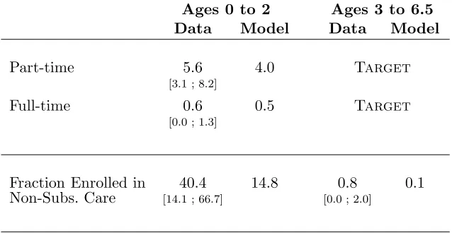
Table 7: Non-Targeted Moments: Child Care Enrollment Rates
Ages 0 to 2 Ages 3 to 6.5 Data Model Data Model
Part-time 5.6 4.0 Target
[3.1 ; 8.2]
Full-time 0.6 0.5 Target
[0.0 ; 1.3]
Fraction Enrolled in 40.4 14.8 0.8 0.1
Non-Subs. Care [14.1 ; 66.7] [0.0 ; 2.0]
Note: 95% confidence intervals for the data moments are given in brackets.
6.1 Child Care Enrollment
In the model two mechanisms are at work that both generate a lower child care enrollment rate for children aged zero to two compared to children aged three to six and a half. First, the utility mothers receive from spending time with their children declines as the children get older. This in turn increases the incentive to use (more) paid and non-paid child care and to participate (more) in the labor market when the children are of ages three to six and a half compared to when the children are of ages zero to two. Second, the cost of using paid child care relative to non-paid child care are higher for children aged zero to two. While the usage of non-paid child care is assumed to be associated with the same utility costs for both pre-school age groups, the utility loss from the usage of paid child care through reduced consumption is very different. Mothers with children aged zero to two who want to use paid child care will mainly have to resort to non-subsidized child care because of the low availability of subsidized child care. In addition, paid child care is more expensive for children aged zero to two: in relative terms because the household income (conditional on the maternal labor force participation status) is on average lower; in absolute terms because subsidized child care fees are on average associated with an extra charge of up to 30% per month,
compare Table C.6in AppendixC.3.
The question is now how well these two mechanisms are jointly able to predict child care enrollment for children aged zero to two. E.g. it could be that the higher costs of paid child care do not matter at all if for working mothers without access to a subsidized slot, the costs of non-subsidized child care are still below the costs of using non-paid child care. As an implication, the predicted child care enrollment rates for children aged zero to two by the model would be much higher than in
the data. The upper panel of Table 7 demonstrates that this is not the case. The two model
Table 8: Non-Targeted Moments: Conditional Child Care Enrollment Rates
Ages 0 to 2 Ages 3 to 6.5 Data Model Data Model
At least part-time care
Not Working 2.9 2.7 93.2 92.1
[0.6 ; 5.1] [87.9 ; 98.7]
Working 13.7 11.6 96.7 96.4
[7.3 ; 20.5] [94.2 ; 99.1]
Full-time care
Full-time Working 3.9 2.7 32.4 28.8
[0.0 ; 11.2] [16.7 ; 47.6]
Note: 95% confidence intervals for the data moments are given in brackets.
care enrollment rate for children aged zero to two in the data.
The model further predicts correctly that for children aged three to six and a half non-subsidized child care is irrelevant. This result is basically implied by the choice of calibration targets, i.e. by matching the part- and full-time child care enrollment rates for this age group at the prevailing provision rates of subsidized child care.
6.2 Conditional Child Care Enrollment
Table 8 shows that the child care enrollment rates conditional on the maternal labor force
par-ticipation status predicted by the model are as well close to the data for both age groups. Very different outcomes for the conditional child care enrollment rates would have also been consistent with matching and explaining the (unconditional) child care enrollment and maternal labor force participation rates. E.g. all and not only 28.8% of the full-time working females with children aged
three to six and a half (8.2 %, see Figure 4) could have been using full-time child care and the
full-time child care enrollment rate (12.9%, see Figure 4) could have been generated by a lower
usage of full-time child care of non- and part-time working mothers.
The successful prediction of the conditional child care enrollment rates cannot be explained by a single mechanism in the model but rather reflects that the main trade-offs mothers face in real life are captured well by the model. Just to give one example: the assignment of subsidized child care slots is random and does not favor working women. This contributes to the relative low full-time child care enrollment rates conditional on working full-time. These outcomes are of course not independent from the costs of non-paid child care (also relative to non-subsidized child care) and the selection into full-time participation.
enrollment choices of mothers, the good predictions of the non-targeted child care moments provide confidence in the model’s explanatory power.
7
Policy Experiments
In April 2008 the German Federal government, back then a coalition of christian (CDU/CSU) and
social democrats (SPD), passed the Kinderf¨orderungsgesetz [Kif¨og]. I evaluate the major parts of
this law that concern the provision of subsidized child care for children aged zero to two.
7.1 Setup of the Reforms
Reform 1: For all children younger than age three a subsidized child care slot shall be provided
from October 2010 onwards if both parents are working. (§24 I 2 and§24a III Sozialgesetzbuch 8)
The bill on the Kif¨og was introduced with the following statement: “Many parents do not realize
their desired fertility level, because of the incompatibility of family and working life ... Therefore it is necessary to improve the compatibility of family and working life. To achieve this, we need
more high quality child care for children younger than age three.” German Federal Parliament
(2008) By this article, the coalition expected to achieve a child care enrollment rate of 35% of all
children younger than age three, and thus compliance with the target of 33% set by the European Commission at its Barcelona meeting in 2002, and to close the gap to the “exemplary standards in Western and Northern European countries, for which a relationship between child care enrollment,
maternal employment and fertility is observed”, see Sharma and Steiner (2008). The reform is
straightforward to implement in the context of the model by conditioning access to subsidized child
care (a1) on the labor force participation status (l1):
a1≥l1. (25)
While full-time working females can always use subsidized part-time or full-time child care, I main-tain the assumption that non-working females rely on the initially specified slot lottery to have access to subsidized child care. Part-time working females are in-between because they can always use subsidized part-time child care but subsidized full-time child care only if they are successful in the slot lottery.
Reform 2: From August 2013 onwards all children of age one and two are entitled to a subsidized
child care slot. (§24 II Sozialgesetzbuch 8)
This passage can be seen in the tradition of providing subsidized child care as a means of af-fordable, high quality pre-school education also for children aged one to two. This view is con-firmed in a dossier of the Federal Ministry of Family Affairs, Senior Citizens, Women and Youth
Sharma and Steiner (2008) accompanying the Kif¨og in which among others the beneficial aspects
Table 9: Policy Regimes
Access Probability (in %) to ... Subsidized Child Care No Part-time Full-time
Ages 0 to 2
Baseline 94.0 ∀l 4.3 ∀ l 1.7 ∀ l
Reform 1 94.0 ifl= 0
0.0 else
4.3 ifl= 0
100.0 else
1.7 ifl≤ 14
100.0 else
Reform 2 0.0 ∀l 100.0 ∀ l 1.7 ifl≤
1 4
100.0 else
Note: l= 0/1 4/
1
2 corresponds to non-/part-/full-time working.
and a half which referred to part-time slots only.21 I therefore assume that the “new” entitlement
also refers to part-time subsidized child care. The actual law applies to all children of age one and two whereas the model period comprises ages zero to two, i.e. one year more. Given the variables
definition employed in Section2and AppendixA.3, access to a subsidized part-time child care slot
for only two years in the data still corresponds to access to a subsidized part-time child care slot for
the whole model period. Hence, Reform 2 will be implemented such that all mothers of children
aged zero to two have at least access to a subsidized part-time child care slot for their children independent of their labor force participation status. Non- and part-time working mothers might still draw from the lottery a subsidized full-time child care slot with the success probability from theBaseline setup.
Table 9 compares the Baseline setup with the previously described reforms. The parental fees for
subsidized and non-subsidized child care are kept at the values of theBaselinesetup.
I evaluate the impact of the reforms in three steps. I first compare the outcome from theBaseline
setup with the two experiments holding the fertility choice fixed, i.e. I ask: how would the females
behave if they had have made their fertility choice under theBaselinesetup but then faced a setup
as described by the respective reforms? This permits to disentangle the direct effect on maternal labor force participation and child care enrollment from the one induced through changes in the fertility choices. In the second step, I discuss the impact of each reform on the fertility choices. Afterwards I summarize the results for the female and maternal labor force participation rates and the child care enrollment rates taking the changes in the fertility outcomes into account and contrast them with case of holding fertility fixed.
21
Note that in theBaselinesetup the total provision rate of subsidized child care for children aged three to six
Table 10: Fixed Fertility - Maternal Labor Force Participation and Child Care Enrollment
Participation Enrollment Part-time Full-time Part-time Full-time
Ages 0 to 2
Baseline 26.5 4.8 4.0 0.5
Reform 1 +3.2 +1.7 +27.3 +6.3
Reform 2 +3.2 +1.7 +53.7 +6.3
Ages 3 to 18.5 (Avg.)
Baseline 60.0 10.8 − −
Reform 1 0.0 0.0 − −
Reform 2 0.0 0.0 − −
Note: The entries for the Baselinescenario refer to the maternal labor force
participation and child care enrollment rates prior toReform 1 and 2. The entries forReform 1and 2 refer to the percentage point changes of the respec-tive maternal labor force participation and child care enrollment rates relarespec-tive to theBaselinescenario.
As a word of caution, the experiments conducted here abstract from any problems in the actual implementation of the reforms. In real life, no one expects the promised subsidized child care slots to be fully available at the date of the implementation of the law. It will rather take a few years until the predictions of the paper maybe contrasted with the empirical data.
7.2 Labor Force Participation and Child Care Enrollment with Fixed Fertility
Table 10 restates the maternal labor force participation and child care enrollment rates from the
Baseline setup and the resulting change in percentage points under each reform. The fertility
choices are held constant at their values from the Baselinesetup.