Munich Personal RePEc Archive
Skill investment, farm size distribution
and agricultural productivity
Cai, Wenbiao
University of Iowa
9 January 2011
Online at
https://mpra.ub.uni-muenchen.de/32806/
Skill Investment, Farm Size Distribution and Agricultural
Productivity
Wenbiao Cai1
Department of Economics, W210 John Pappajohn Business Building, Iowa City, IA 52242-1000.
Abstract
Cross-country differences in agricultural productivity dwarf those in the aggregate. This
pa-per presents a theory in which low aggregate productivity distorts skill formation of farmers.
A model in the style of Lucas (1978) is extended to allow skill accumulation. Differences
in skill magnify the differences in agricultural productivity. The model is calibrated to the
U.S. to reproduce the size distribution of farms and the time allocation of farmers. Given
exogenous differences in total factor productivity (TFP), the model explains 45-50% of the
differences in agricultural output per worker. Moreover, differences in farmers’ skills account
for about 30% of the variation in agricultural productivity. The model also maps the latent
distribution of skill to a size distribution of farms, and is able to resemble salient features of
the cross-country distribution of farm size.
Keywords: Agricultural productivity, skill investment, farm size distribution, income
differences.
1. Introduction
Cross country differences in agricultural productivity are much larger than the differences
in aggregate income per worker. This feature is first noted in Kuznets (1971). For a larger
1
set of countries, Caselli (2005) documents that between the 90th percentile country and the
10th percentile country of the world income distribution, the ratio of PPP output per worker
in agriculture exceeds a factor of 45, compared to 22 in GDP per worker and merely 5 in
non-agricultural output per worker. Given that agriculture typically employs most of the
labor force in low income countries, understanding why agriculture is so unproductive in
these countries is clearly of first order importance.
This paper presents a theory in which unmeasured skill of farmers plays an important role
in agricultural production. I construct a model featuring an agricultural sector displaying
decreasing returns to scale, and a non-agricultural sector displaying constant returns to scale.
Skill is modeled as the ability to manage a farm, in the style ofLucas(1978). Given the same
amount of input, a more skilled individual is able to produce more agricultural output. Hence
agricultural productivity critically depends on the skill component of individuals who choose
to become farmers and produce in agriculture. Such division of labor between occupations
arises endogenously in equilibrium. Moreover, it is shown to vary with the level of aggregate
productivity.
The model also features growth of skill in a life cycle set up. On the one hand, the
dynamics of skill bring about an addition margin through which TFP affects productivity in
agriculture. On the other hand, such specification accords well with micro farm level data
in the U.S.. While detailed description of the data is postponed until Section 2, the key
observation is that productivity of a US farm operator can grow as much as by a factor of 3
over her life cycle. This life-cycle feather is robust to different ways of measuring productivity.
In this paper, productivity growth is not viewed to be a mere byproduct of working and
aging. Instead, it is the result of explicit skill-enhancing investment committed earlier in a
farmer’s life. In fact, younger farm operators in the US tend to spend more time on non-farm
activities, relative to their older peers. Consistent with these empirical observations, a skill
investment over their life cycle, in addition to their selection of occupations.
The key result is that economy with low TFP comprises of a large pool of low skill
farmers. In a high TFP economy, farmers are rare but possess high skill. This is true despite
the fact that economies differ only in their levels of TFP, which is sector-neutral. Moreover,
the differences in the skill composition of farmers arise from two distinct margins. Through
the extensive margin, the subsistence need of agricultural good dictates that more people,
even those with low skill, produce in agriculture. To the extent that a low-skill farmer can
be viewed as having a comparative advantage in non-agriculture, this margin is similar to
the “specialization” effect inLagakos and Waugh(2010). The authors show that subsistence
need induces less specialization in low TFP countries, and offer a neat explanation of
cross-country productivity differences at the sector level. The intensive margin operates through
on-the-job skill investment. Farmers in a low TFP economy invest less in skill improvement
due to high financing cost - in the form of high equilibrium interest rate. In addition to a
larger pool of farmers, each farmer faces a flatter life-cycle skill profile in such an economy.
Skill accumulation hence offers an extra channel through which TFP affects the skill of
farmers (and consequently productivity in agriculture), and is a key innovation of this paper.
The intensive margin is particularly interesting. In a standard human capital model with
only time input in the human capital technology, it is generally the case that difference
in the level of TFP has no impact on the optimal allocation of time. Recent advances in
the literature stress the key role of goods input in the human capital technology. Excellent
examples along this line include Manuelli and Seshadri (2005), Cordoba and Ripoll (2007),
and Erosa, Koreshkova, and Restuccia (2010). In these papers, goods input contributes to
the differences in the “quality” of human capital. In the current paper, goods input is absent
in the skill accumulation technology. Nonetheless, optimal time investment varies with the
level of TFP. This is because low TFP is accompanied by high equilibrium interest rate,
When fed exogenously the level of TFP and land endowment, the model has predictions
about the allocation of labor across sectors, time allocation of farmers between investment
and production, and output per worker in agriculture and non-agriculture. In equilibrium,
the model also yields a non-degenerate size distribution of farms. This is particularly useful
because there is a unique mapping between the distribution of farmer’s skill and the size
distribution of farmers. Hence the model’s prediction about cross-country difference in skill
of farmers can be tested by investigating its implication about the size distribution of farms
across countries.
To be used to explain cross-country differences in agricultural productivity, the model is
calibrated to the US as a benchmark economy. In particular, model parameters are chosen
such that the model reproduces the size distribution of farms, time allocation of farmers, and
other macroeconomic statistics in the US. By varying country-specific TFP to reproduce PPP
output per worker in non-agriculture, the model is able to explain 45-50% of the variation in
agricultural output per worker across countries. While cross-country difference in agricultural
productivity is mostly a story of TFP difference - difference in TFP accounts for 50% of the
productivity difference - the importance of skill is too large to ignore. The difference in skill
of farmers is found to account for 27% of the difference in agricultural productivity. Further
decomposition reveals that most of the variation in skill stems from the extensive margin.
While farmer do differ in their accumulation of skill, the difference is quantitatively small.
Consistent with the prediction that farmers possess low skill in low TFP countries, the
model predicts that farms are much smaller in size in those countries. This prediction is
well supported by data on the size distribution of farms across countries. In the data, the
correlation between PPP output per worker in agriculture and mean farm size is 0.45. In
the model, it is 0.6. The model also successfully captures the fact that farms in low income
countries are predominantly small. For the poorest 5% countries, for example, the share
of 87%, which is almost identical to that in the data. For some individual countries, the
endogenous size distribution of farms almost perfectly matches their empirical counterpart.
On the prediction of cross-country size distribution of farms, this paper is related to
Adamopoulos and Restuccia (2011). Both papers use a span-of-control framework to
pro-duce a nondegenrate size distribution and aim at explaining international productivity
difference in agriculture. However, there are subtle yet important differences. Firstly,
Adamopoulos and Restuccia (2011) offers an alternative, and interesting, application of the
span-of-control framework. In particular, they do not consider the division of heterogeneous
family members into different occupations. Such specification allows them to isolate the
ef-fect of idiosyncratic policy distortions on total output in agriculture. As a result, the origins
of productivity differences are not the same in these two papers. In their paper, productivity
is low in agriculture because the most productive farms are not operating at the optimal
scale, due to distortions. In the current paper, low productivity is due to a large share of
unproductive farmers who do not invest to enhance their skill. All farmers, productive or
not, are producing at their optimal scale. Secondly, these two papers also differ in their
implications of the farm size distribution. In Adamopoulos and Restuccia (2011), the size
distribution of farms is used to infer the distribution of idiosyncratic policy distortions. In
this paper, the size distribution is a mapping from the distribution of farmer’s skill. Hence
the difference in the size distribution of farms reveals information about the difference in the
skill composition of farmers.
This paper fits into an expanding literature that emphasizes the key role of
agricul-ture in understanding cross-country productivity differences. Within development
account-ing frameworks, researchers found that includaccount-ing an agriculture sector yields different
im-plications about cross-country difference in TFP than those from the one-sector models.
Cordoba and Ripoll (2005), Chanda and Dalgaard (2008),Vollrath (2009) are excellent
sec-tor productivity in general equilibrium models. Gollin, Parente, and Rogerson (2004) show
that in a model with home production, investment distortions reduce measured
productiv-ity much more in agriculture, relative to non-agriculture. Restuccia, Yang, and Zhu (2008)
argue convincingly that barriers to intermediate inputs in agriculture can substantially
re-duce productivity. High transportation cost is shown to adversely impact productivity in
Adamopoulos (2006) and Gollin and Rogerson (2010). Instead of modeling specific
distor-tions, this paper considers the effect of low aggregate TFP on agricultural productivity in a
model of heterogenous producers. In modeling unmeasured skill in agricultural production,
this paper also relates to Assuncao and Ghatak (2003). However, they mainly focus on the
inverse correlation between farm size and land productivity.
The remaining of the paper is organized as follows. Section 2 presents a set of facts
that motivate this paper. Section 3 describes the economic environment. Section 4 defines
a competitive equilibrium, elaborates on equilibrium conditions, and proves some results.
Section 5 presents the calibration strategies and the main results. Section 6 concludes. All
proofs are relegated to the Appendix.
2. Facts
The main source of data is Census of Agriculture of various years in the US. The unit
of observation is the average of all farms under the management of operators in a particular
age group. First, I show that there is substantial productivity variation across operators of
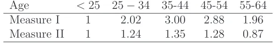
different ages. Two measures of productivity are constructed, and presented in Table 1. In
both measures, the productivity of the youngest operator is normalized to unity. Measure
I is output (net of government transfer) per operator. With measure I, older farmers are
significantly more productive than their younger peers - the productivity gap is as large
as a factor of 3 between operators aged 35-44 and those under 25. While it is true that
ob-served productivity difference can not be completely accounted for by differences in factors
of production. I consider four factors of production: intermediate inputs, land, capital, and
hired labor. Intermediate inputs include feed, seed, chemical and fertilizers. Capital
in-cludes machinery, equipments, and buildings.2 The elasticities of each factor of production
are calculated from Table 5 and 6 in Herrendorf and Valentinyi (2008). Then productivity
is computed as a residual and reported as Measure II in the last row of Table 1.3 Operators
aged 35-44 remain 35% more productive than those under 25. In summary, both measures
of productivity suggest substantially variation across operators of different ages.
[image:8.595.167.443.319.363.2]Age <25 25−34 35-44 45-54 55-64 Measure I 1 2.02 3.00 2.88 1.96 Measure II 1 1.24 1.35 1.28 0.87
Table 1: Productivity By Age of Operator: US (2007)
Perhaps not surprising, older farmers also operate a larger farm. The average size of
farms under the management of operators under 25 is 324 acres, which is about 1/3 the
mean size of farms managed by operators aged 35-44. If one computes output per worker
by size of a farm, it is likely that a larger farm will have higher measured productivity than
a smaller one. In fact, this observation has been highlighted in Adamopoulos and Restuccia
(2011) for the US, and in Cornia (1985) for a larger set of developing countries.
It is also possible that the observed cross-section productivity differences reflect
differ-ences in education attainment of operators. Unfortunately, education attainment is not
reported in the census of agriculture. Instead, I offer indirect evidence suggesting that
ed-ucation attainment is not likely to be the story behind these productivity differences. I
compute operator’s productivity using measure I with data from 1997 and 2002 census of
2
Census reports value of land and buildings. I assume an equal split between land and buildings. The results change minimally with different shares.
3
Solow residual of operatoriis computed as yi
kαk i ·xαxi ·ℓ
αℓ i ·h
αh i
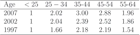
agriculture. The results are reported in Table 2. For the moment, assume that in 1997 the
productivity difference between operators aged 25-34 and those aged 35-44 are driven solely
by education attainment. Then in the 2007 cross section, one should expect to observe the
same order of difference in productivity between operators aged 35-44 and those aged 45-54,
because education attainment is fixed over time. However, We donnot observe that. Similar
calculations for other age groups deliver similar results. Although this calculation is simple
in nature, and in particular ignores the entry of farmer (who might have different education
than the incumbents) over time, it does suggest that the difference in level of education is
not likely to account for, at least not completely, the difference in productivity.
[image:9.595.186.427.338.398.2]Age <25 25−34 35-44 45-54 55-64 2007 1 2.02 3.00 2.88 1.96 2002 1 2.04 2.39 2.52 1.86 1997 1 1.66 2.18 2.19 1.54
Table 2: Productivity by Age of Operator: US (Various Census Years)
International data on productivity by the age of farm operators is limited, especially
for developing countries. Here I present summarized information for one country, Nepal,
that has available data in a similar format as that in the US. Instead of measuring output,
census of agriculture in Nepal (2001-2002) reports average holding size by age of holders,
which I take as a proxy for productivity. In Table 3 I report the mean farm size relative
to that of holders aged less than 25, in both Nepal and the US. The key message to take
away is that productivity growth over farmer’s life cycle is less pronounced in Nepal than in
the US. Between operators aged under 25 and those aged 35-44, the gap in productivity is
around a fact of 1.2 in Nepal, compared to 2.7 in the US.4 This observation is closely related
to the findings in Hsieh and Klenow (2011). The authors find that in the cross-section of
manufacturing plants, surviving plants grow faster in the US, compared to those in Mexico
4
and India. As a result, the life-cycle profile of employment appears flatter in Mexico and
India.
Holding Size <25 25−34 35-44 45-54 55-64
US 1 1.77 2.65 2.81 2.27
[image:10.595.163.449.170.217.2]Nepal 1 1.05 1.2 1.46 1.59
Table 3: Holding Size by Age of Holder: Nepal and US
3. Model
3.1. Environment
Each period a continuum (of measure one) of individuals are born, and live for T periods.
Individuals of the same cohort form a household, with all decisions made by a hypothetical
household head. Two goods are produced each period. One is labeled agricultural good,
denoted byca. The other is labeled non-agricultural good, denoted bycn. The representative
household derives utility from consumption of two goods according to
U(ca, cn) = η·log(ca−¯a) + (1−η)·log(cn)
Parameter ¯a is the subsistence in agricultural consumption. ¯a > 0 implies an income
elas-ticity of agricultural consumption less than unity.
Each member is endowed with one unit of physical time. The fixed stock of land, denoted
by ¯L, is equally owned by households. There is no population growth or lifetime uncertainty.
Total measure of population at any point in time is T.
3.2. Skill Accumulation
When born, individuals within a household draw independently their skill type, z ∈ ℜ+,
from a known, time invariant distribution G(z). Throughout the paper, an individual with
skill can grow over time. And the growth of skill requires investment of time according to
the following technology
zt+1 =zt+zt·sθt, st∈[0,1] (1)
where st is the fraction of time committed to skill enhancing activities. It is not
diffi-cult to map Equation (1) to farming in the real world. To improve skill, a farmer has
to spend time on various tasks including, but not limited to, experimenting with
differ-ent seeds/crops/fertilizers, updating on the most recdiffer-ent available technologies, learning new
equipments etc. While other skill-enhancing tasks may require input other than time - e.g.,
purchasing a new computer, such possibilities are ruled out here for several reasons. First,
it allows for closed-form solutions and clearer expositions. Second, data on time allocations
of farm operators are available to discipline relevant parameters. Lastly, data on resources
investment by farm operators in skill accumulation are limited, if available at all.
3.3. Technology and Household Optimization
Conditional on skill type, the household head decides whether a member should be a
worker or a farmer. This division of labor is assumed to be fixed over one’s life. This
re-striction is innocuous in a steady state. All workers, regardless of skill type, supply labor
inelastically and earn a common wage. A farmer produces agricultural goods using a
tech-nology displaying decreasing returns to scale, and retains profit as rent. The techtech-nology is
standard Cobb-Douglas
ya =A·(z(1−s))1−γ hα a ·ℓ
1−αγ
level of total factor productivity in this economy.
There are competitive rental markets of labor and land at prices w and q, and farm
output are sold in competitive markets at price p. All prices are expressed relative to the
price of nonagricultural output. In a given period, a farmer with skill level z who works
(1−s) hours rents labor and land to maximize profit
max
{ha,ℓ}
p·ya−w·ha−q·ℓ
For later reference, denote ha(z, s), ℓ(z, s) the optimal demand of labor and land. The
profit, denoted by π(z, s), is retained by the farmer as rent. It is straightforward to show
that profit is linear in the skill input, i.e.,
π(z, s) =z(1−s)·(1−γ)·(p·A)1−1γ γ
α
w
α1−α q
1−α!
γ
1−γ
LetYtdenote household income in period t, given the division of labor and the allocation
of time between skill accumulation and production. The household head then solves the
standard consumption-saving problem to maximized discounted utility
max
{cat,cnt}
:
T
X
t=1
βtU(cat, cnt)
s.t: ptcat+cnt+at+1 =atRt+Yt
3.4. Non-agriculture
There is a representative firm that produces non-agricultural output with a linear
tech-nology Yn =A·Hn. In this technology, Hn denotes labor hours and does not embed skills.5
The representative firm solves
max
{Hn}
A·Hn−w·Hn
4. Equilibrium
This economy admits a stationary equilibrium, in which prices and the division of labor
are constant over time. A formal definition is given below.
A stationary competitive equilibrium is a collection of prices (w, p, q, R), consumption
and investment allocations (cat, cnt, st, at)T
t=1, factor demand ha(z, s), ℓ(z, s), Hn such that:
(1) given prices, (cat, cnt, st, at)Tt=1 solve household maximization problem; (2) given prices,
ha(z, s), ℓ(z, s)solve farmer’s profit maximization, andHnsolve non-agricultural firm’s profit
maximization; (3) prices are competitive; (4) all markets clear.
In equilibrium, workers work full time because the return to skill investment is zero. The
discounted lifetime income of a worker is simplyYw =PTt=1{w·R1−t}. Since farmer’s rent is
strictly increasing in skill input, it is always profitable for a farmer to spend positive amount
of time on skill accumulation. Moreover, the optimal time investment is independent of
farmers’ skill type. Lemma 1 states this result formally.
Lemma 1. Optimal time investment is independent of initial skill draw
Lemma 1 implies a common slope of skill profile for all farmers, and the level is determined
5
Alternatively, the technology can be specified as y = ARizidGito incorporate skill. In this case, the
by the initial draw. It is convenient to define variable xt as follows
xt =
1, t= 1
xt−1·(1 +sθt−1), t= 2, ..., T
{xt}T
t=1 summarize the level of skill at time t relative to the initial draw. Clearly, {xt} is
independent of skill type. This allows a simple expression of lifetime discounted income of a
typez farmer
Yf(z) =π(z)·
T
X
t=1
{xt·(1−st)·R1−t}
Note thatYf(z) is linear and strictly increasing in skill typez. Recall that discounted lifetime
income of a worker (Yw) is independent of skill type z. This leads to Lemma 2.
Lemma 2. There exists a cut-off level of skill type, z¯, such that household members with skill typez <z¯become workers, and household members with skill typez >z¯become farmers.
The most able members will manage farms and utilize their skills. The less able members
will supply inelastically one unit of labor to the market, and forgo their endowed skills. The
marginal farmer, whose skill type is ¯z, is indifferent between two occupations. Income of a
household consists of labor income, farm profit, and rental income from land. The present
value of household income is simply
Y =G(¯z)·Yw+
Z
¯
z
Yf(z)dG(z) +q·L/T¯ ·
T
X
t=1
R1−t
To solve the model, I begin by solving for prices (p, q). Equation (2) below states the
clearing condition, which utilizes the fact that land demand is linear in skill input.
π(¯z)·
T
X
t=1
{xt·(1−st)·R1−t}=
T
X
t=1
{w·R1−t} (2)
Z
¯
z
ℓ(z)dG(z)·
T
X
t=1
{xt·(1−st)}= ¯L (3)
Dividing (2) by (3) yields an expression for the rental price of land
q=
" PT
t=1{xt·(1−st)}
PT
t=1{xt·(1−st)·R1−t}
#
·
γ·(1−α)·PTt=1{w·R1−t}
(1−γ)·L¯
· R
¯
zzdG(z)
¯
z (4)
Substituting (4) into (3) yields the relative price of agricultural good
p=
" PT
t=1{w·R1−t}
¯
z·(1−γ)·PTt=1{xt·(1−st)·R1−t}
#1−γ
· γα w
α1−α q
1−α!−γ
· 1
A (5)
Note the relative price of agricultural good is strictly decreasing in TFP. Agricultural good
is more expensive relative to non-agricultural good in countries with low productivity.
Solv-ing for optimal consumption bundles and aggregatSolv-ing over generations yields the aggregate
demand of two consumption goods
Ca = T X t=1 cat = " T X t=1
(βR)t−1
#
·
"
Y −p·¯aPTt=1R1−t
PT t=1βt−1
#
· η
p +T ·¯a (6)
Cn = T X t=1 cnt = " T X t=1
(βR)t−1
#
·
"
Y −p·¯aPTt=1R1−t
PT t=1βt−1
#
·(1−η) (7)
In each household, the measure of workers is G(¯z). Given constant prices, the division
of labor does not change across cohorts. Hence the total measure of worker in the economy
by first integrating over farmers within a household, and then summing over generations
Ha=
" T X
t=1
xt(1−st)
#
·
Z
¯
z
ha(z)dG(z)
Similarly, aggregate agricultural output is given by
Ya =
" T X
t=1
xt(1−st)
#
·
Z
¯
z
ya(z)dG(z)
Imposing labor market clearing, the measure of workers in the nonagricultural sector is
Hn=T·G(¯z)−Ha. The output in the nonagricultural sector isYn=A·Hn. Goods market clearing conditions require Ca=Ya, Cn =Yn. Loan market clears by Walras’ law.
Finally nonagricultural firm’s optimization implies w=A. Hence the two goods market
clearing conditions constitute two equations with two unknowns (¯z, R) that can be solved
numerically. Once the cut-off skill and interest rates are known, rest of the equilibrium
variables can be recovered easily. Proposition 1 states an important result.
Proposition 1. Economy with lower TFP has a lower cut-off skill level, and a higher in-terest rate.
Proposition 1 implies that low aggregate productivity adversely impacts the productivity
of farmers through both the extensive margin and the intensive margin. On the one hand,
due to subsistence, low TFP necessitates a larger pool of farmers. Moreover, the selection of
farmers implies that more entrance is associated with a decline in the average productivity
of farmers. On the other hand, financing skill investment is more costly in a low TFP
economy. High interest rate renders increase in future income less attractive. As a result,
the skill profile is less steep. Both margins lead to lower average productivity of farmers,
5. Quantitative Analysis
5.1. Calibration
In this section the model is parameterized to answer quantitative questions. Individuals
are born at the age of 25 and live for 5 periods. Each period corresponds to 10 years.
Some model parameters are either standard or can be inferred without solving the model.
Assuming an annual discount rate of 0.96, I setβ = (0.96)10. For the US, TFP is normalized
to be 1.6 The endowment of land is approximated by the arable land (in hectares) per
worker. To pin down parameters in the agricultural technology, I turn to value added data
in agriculture. Over the period 1980-1999, the average share of agricultural output accruing
to farm operators is 40%, implying γ = 0.6. Given this value, parameter α is chosen such
that labor share (αγ) is consistent with the ones estimated in Hayami and Ruttan (1970).
This paper is certainly not the first one to estimate the span-of-control parameter.
How-ever, existing works either focus on the aggregate economy as in Guner, Ventura, and Yi
(2008) andRestuccia and Rogerson(2008) or the manufacturing sector as inAtkeson and Kehoe
(2005) and Gollin (2008). The value of the span-of-control parameters from these studies
range from 0.8 to 0.9. To my best knowledge, there is no consensus on the range of this
parameter in the agricultural sector. A value of 0.6 for agriculture is nevertheless a
conser-vative choice as a higher γ tends to strengthen the quantitative results. Section 5.3 provides
more detailed discussion about the choice of this parameter.
Exogenous skill type distribution is assumed to take a log-normal form with mean µand
standard deviationσ. Given values of (β, A, γ, α), the remaining six parameters (¯a, η, µ, σ, θ)
are chosen simultaneously to match moments of the US economy in 1985. From the World
Development Indicator, agriculture employs 3% of the labor force. Following the strategies in
6
Restuccia, Yang, and Zhu (2008) , η is chosen to target a long run agricultural employment
share of 0.5%. This corresponds to the asymptotic agricultural employment share when the
subsistence consumption share of income is effectively zero. Parameter θ governs the time
allocation between skill accumulation and production. Direct observation on the time split
between these two activities are not available. However, the model implies that farmers
of generation i spend (1−si) fraction of labor hours producing in their farms. Hence the cross-section distribution of hours supplied by operators of different ages is simply given by
1−si
PT
i=11−si. Census of agriculture reports working days of farmers in 5 different age groups:
25-34, 35-44, 45-54, 55-64, 65+, which allows me to calculate the distribution of hours in the
data. I chooseθ to best match the empirical distribution. Finally, the model is calibrated to
reproduce the observed size distribution of farms in the US. Figure B.4 plots the calibrated
size distribution against data. In addition, as depicted in Figure B.5, the model also implies
a land distribution that fits the data very well, even though it is not targeted. These figures
are presented in Appendix B. Table 4 offers a summary of parameter values and how they
are selected.
Parameter Description Value Source
A TFP 1 Normalization
T Life cycle 5 Model period = 10 years. Born 25, die 75
β Discount (0.96)10
Common value ¯
L Land endowment 1.62 Arable land per worker
γ Span-of-control 0.6 Income share of farm operator
α Labor share, agriculture 0.8 Hayami and Ruttan(1970)
η Expenditure share, agriculture 0.01 Restuccia, Yang, and Zhu(2008) ¯
a Subsistence 0.2 Share of labor in agriculture
θ Time elasticity in skill accumulation 0.33 Hour distribution of farmers
µ Skill distribution, mean −2.45 Size distribution of farms
[image:18.595.72.540.478.625.2]σ Skill distribution, stdev 4.16 Size distribution of farms
Table 4: Parameter Description, Value, and Source of Identification
5.2. Results
Our sample consists of 50 countries with complete information on sector output per
are directly available from Restuccia, Yang, and Zhu (2008). The last is compiled from the
World Census of Agriculture, a database maintained by the Food and Agriculture
Orga-nization. These two sets of data, however, are not directly comparable because of time
period differences. The data in Restuccia, Yang, and Zhu (2008) pertain to the year 1985.
World Census of Agriculture is a collection of national agriculture censuses administered
independently in each member country - possibly in different years. Most of the countries
indeed have their censuses conducted around 1990, and hence can serve as good proxies. It
is unlikely that the composition of farms will undergo drastic changes over a period of five
years.
Countries differ in their Total Factor Productivity (A) and land endowment ( ¯L), and
are otherwise identical. The central question of interest is to quantitatively assess how
differences in aggregate productivity (and endowment) affects the skill of farmers, and
con-sequently agricultural productivity. This inquire falls along the line with those in Gollin
(2008) andLagakos and Waugh (2010). The former asks how aggregate productivity affects
the composition of labor across countries, and the latter explores how differences in aggregate
efficiency can translated in to asymmetric differences in sector labor productivity. Countries
are assume to face the same distribution of skill types ex-ante. Finally, utilizing the linear
technology in non-agriculture, TFP of country i can be inferred as
Ai = ynlni
ynlnus
where ynlni is PPP non-agricultural GDP per worker of country i.
How does the model perform in explaining cross-country variation in agricultural
produc-tivity? Two statistics are constructed to help answer this question. The first one, following
Caselli (2005), computes the ratio of log-variance of model generated productivity series to
variation in agricultural output per worker across 50 countries. The second one is the R2
statistics of OLS regression of model series on data. A very similar value (0.49) is obtained.
Figure1 plots model agricultural productivity against that in the data, both re-scaled such
that productivity in the US is equal to unity. A visual outlier is Nepal, for which the model
over-predicts its agricultural productivity by a lot. The reason is that Nepal, despite a very
high employment share in agriculture, has a very productive non-agricultural sector. This
maps into high TFP, and leads to a counterfactually high productivity in agriculture.
1/128 1/64 1/32 1/16 1/8 1/4 1/2 1 1/128 1/64 1/32 1/16 1/8 1/4 1/2 1 BFA UGA NPL SEN IND CIV PHL PAK BGD IDN HND THA NIC PRY MAR DOM TUR EGY PER TUNCOL
ECU CHL URY KOR HUN BRA PRT ARG GRC VEN JPN IRL ESP GBR FIN
AUT DNK NZL SWEFRAITA
DEU BELNLD NOR
AUS
CHE
CAN USA
← 45o Line
PPP Agricultural Output per Worker: Data
PPP Agricultural Output per Worker: Model
[image:20.595.145.460.301.463.2]Agricultural Productivity: Model and Data
Figure 1: Agricultural Productivity: Model and Data
Low agricultural productivity is mainly due to low total factor productivity, as opposed
to deficiency in land endowment. Consider, for concreteness, the poorest country in the
sample (Burkina Faso). Compared to the US, Burkina Faso is 4.8 times less productive
overall and has 2.6 times less land per worker. Imagine that Burkina Faso has the US
land endowment, but its own TFP. This can not help Burkina Faso catch up with US in
agricultural productivity - the gap shrinks from a factor 28 to 22. If, however, Burkina
Faso has the US level of TFP and its own land endowment, its productivity in agriculture
is increased big time - the gap shrinks to merely a factor of 1.2. Productivity differences
across countries is mainly a story of TFP differences. This is true not only at the aggregate
agriculture.7
It is worth pointing out that countries in the sample do not differ a lot in terms of PPP
output per worker in non-agriculture. Between US and the least productive country, the gap
does not exceed a factor of 6. As a result, countries are not assumed to differ a lot in terms of
aggregate TFP in the quantitative analysis. Hence, the much larger productivity differences
in agriculture generated from the model are not manufactured exogenously, but rather reflect
the mechanisms highlighted in the paper, namely, low TFP produces a large pool of unskill
farmers, which produce on small scale and low efficiency. For a clearer exposition, first note
that total output in agriculture can be written as
Ya =A·
T
X
t=1
xt(1−st)·
Z
¯
a
zdG(z)
!1−γ
· Hα a ·L¯
1−αγ (8)
Let M denote the measure of farmers, then output per worker is simply yala = Ya
M+Ha.
Substituting equation (8) into this expression and rearranging terms yields the following
expression of agricultural productivity
yala= A
|{z}
T F P
·
T
X
t=1
xt(1−st)
!1−γ
| {z }
Intensive Margin
·(E(z|z >z¯))1−γ
| {z }
Extensive Margin
· L¯(1−α)γ
| {z }
Land Per Worker
· (Ha)
αγ·M−γ
1 +Ha/M
| {z }
Labor Composition
·Tγ−1 (9)
Equation (9) offers a nice decomposition of output per worker in agriculture. First of all,
Low TFP and poor land endowment decreases agricultural productivity directly. Moreover,
TFP also affects the skill profile of farmers, and does to through two distinct margins. The
term E(z|z > z¯) is the average skill type of farmers, and captures the extensive margin. As more and more farmers produce in agriculture, the average skill is driven down because
7
the marginal farmer is less and less productive. The term PTt=1xt(1−st) summaries the steepness of the skill profile, and captures the intensive margin. By proposition 1, both
terms increase with aggregate productivity, and leverages the impact of TFP on agricultural
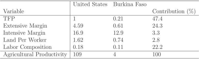
productivity. To quantify the contribution of each component, consider again the comparison
between Burkina Faso and the US. The last column of Table 5reports how each component
contributes to the agricultural productivity differences between these two countries.
United States Burkina Faso
Variable Contribution (%)
TFP 1 0.21 47.4
Extensive Margin 4.59 0.61 24.3
Intensive Margin 16.9 12.9 3.3
Land Per Worker 1.62 0.74 2.8
Labor Composition 0.18 0.11 22.2
[image:22.595.103.509.270.390.2]Agricultural Productivity 109 4 100
Table 5: Decomposition of Agricultural Output per Worker
Between these US and Burkina Faso, differences in TFP explain about 50% of the
differ-ences in agricultural output per worker. Differdiffer-ences in farmer’s skill, extensive margin and
intensive margin combined, explains about 30% of the differences in agricultural
productiv-ity. Most of the variation in farmer’s skill comes through the extensive margin. Exogenous
differences in land endowment accounts for less than 3% of the differences in agricultural
productivity. The results also suggest that these two countries differ substantially in the
composition of agricultural workers. In addition to operating with a bigger plot of land,
each farm in high TFP countries employs more worker. This appears consistent with the
observation the majority of farms in poor countries are small family farms, with limited
input of hired labor.
Given its latent nature, differences in farming skill are unobservable to an economist.
Instead of trying to construct reasonable measures of farming skill from the data, a different
distribution of skills and the size distribution of farms. Although the former is not observable,
the latter is. Moreover, more skilled farmers operate a bigger farm, other things equal. Hence,
two observations should follow if farmers in poor countries indeed have lower skill. First,
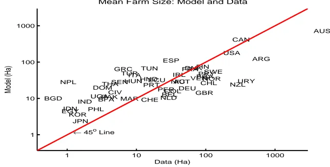
mean farm size should be smaller in poor countries. Indeed, it is. A typical farm in Burkina
Faso is only 1/20 the size of a typical farm in the US. Figure 2 plots mean farm size in the
model and in the data. The model successfully reproduces the positive correlation between
output per worker in agriculture and mean farm size. In the Appendix, the size distributions
of some selected countries are plotted against their empirical counterparts. Although the
model is not expected to replicate the empirical distribution exactly, it does reproduce one
salient feature of the data, namely, the size distribution of farms in low income countries
is more skewed to the left. This comes from the fact the there is a larger share of low
skill farmers in these countries. The discrepancy between the model distribution and the
empirical distribution - the part that a model of skill investment is unable to explain - might
imply farm level distortions that are prevalent in developing countries8 and highlighted in
Adamopoulos and Restuccia (2011).
1 10 100 1000
1 10 100 1000 BFA UGA NPL SEN IND CIV PHL PAK BGD IDN HND THA NIC PRY MAR DOM TUR EGY PER TUN COL ECU CHL URY KOR HUN BRA PRT ARG GRC VEN JPN IRL ESP GBR FIN AUT DNK NZL SWE FRA ITA DEU BEL NLD NOR AUS CHE CAN USA
← 45o Line
Data (Ha)
Model (Ha)
[image:23.595.144.466.490.653.2]Mean Farm Size: Model and Data
Figure 2: Mean Farm Size: Model and Data
8
Agriculture, despite its low productivity, absorbs most of the labor force in poor nations.
The model performs less well explaining this stylized fact. Figure 3 plots the share of
agricultural labor in the model and in the data. For low income countries, the model generally
predicts a smaller agricultural labor share than in the data. This is not surprising given that
the model is a highly stylized one. It is not at all difficult to list features that can generate
a larger share of agricultural labor if included in the model. Among other things, barriers
to sectoral labor movements are particularly important to the question posted here. Such
barriers are prevalent in developing nations as evidenced by substantial disparities in
rural-urban earnings. One famous example is theHukousystem in China that imposes institutional
restrictions on immigration from rural villages to urban cities. However, accurate measures
of such distortions might be difficult, if at all possible, to obtain for a large set of countries,
making the quantitative analysis less rewarding.
0 0.2 0.4 0.6 0.8 1
0 0.1 0.2 0.3 0.4 0.5 0.6 0.7 0.8 0.9 1 BFA UGA NPL SEN IND CIV PHL PAK BGD IDN HND THA NIC PRY MAR DOM TUR EGY PER TUNCOLECU CHLURYHUN KOR
BRA PRT ARGVEN GRC JPN
IRL ESP GBRSWEDEUDNKFRAAUTITAFINNZL BELUSACANNLDCHEAUSNOR
45o Line →
Data
Model
[image:24.595.153.455.420.580.2]Share of Worker in Agriculture: Model and Data
Figure 3: Share of Worker in Agriculture: Model and Data
Agriculture’s share of total output declines as income rises - a macroeconomic implication
of Engel’s Law. The model predicts agricultural output to be 10% of the aggregate output
in the top quintile countries, and 70% in the bottom quintile countries. In the data, the
value is 3% and 30%, respectively. One possible explanation is that the model over-predicts
when measured at domestic prices. Using ICP data from the World Bank, I compute the
relative price between “agricultural consumption” and “nonagricultural consumption” for all
available countries.9 The relative price in 2005 is around 4 times higher in the 10th percentile
country, compared to the 90th percentile country. In the model, this relative price ratio is
2.8, which is roughly in line with the data.
5.3. Discussion
The model presented in the current paper is a stylized one. In this economy,
farm-ing is the job with the highest return. This is at clear odds with the data, even in the
most agriculture-advanced countries like the US. However, the focus of this paper is the
cross-country comparison of agricultural productivity. It intends to provide an explanation
of why one country is less productive in agriculture relative to another country. In this
respect, missing the level of agricultural productivity does not invalidate the comparison
across countries.
The key contribution is to present a framework that embeds skill accumulation in a
span-of-control model framework. One the one hand, this specification allows a mapping from
the equilibrium distribution of skills to the observable size distribution of farms, making
model predictions verifiable. On the other hand, while skill investment is not essential
to this mapping in the sense that a non-degenerate size distribution aries even without
skill investment, it is critical to the identification of the underlying skill distribution in the
benchmark economy. A model without skill investment fails to reproduce the farm size
distribution of the US, at least within the family of log-normal skill distributions. A similar
finding is reported in Bhattacharya (2009), who shows that skill accumulation is critical to
quantitatively explain cross-country variation in firm size distribution and income.
9
The span-of-control parameter is key to the quantitative results. A higher value of γ
implies sharper differences in the division of labor in response to given differences in aggregate
productivity. As discussed before, existing estimates of this parameter for the manufacturing
sector or the aggregate economy are typically in the ballpark of 0.8. In this respect, the
preferred value of 0.6 is a conservative choice. To illustrate this, the model is re-calibrated
under the case of γ = 0.8. Then I ask again how much of the differences in agricultural
productivity between the US and Burkina Faso can be accounted for by the model, given
exogenous TFP and land endowment. The results are summarized in Table 6.
United States Burkina Faso Gap
γ = 0.6 109 4 27
γ = 0.8 15.7 0.49 31
[image:26.595.182.430.319.381.2]Data 19930 128 155
Table 6: Agricultural Productivity Differences Under Differentγ
The model is able to explain 15% more of the differences in agricultural productivity
between US and Burkina Faso when a largerγ is chosen. However, the relative contribution
of exogenous and endogenous variables remains more or less the same. With γ = 0.8, TFP
accounts for 45% of the differences in agricultural productivity, followed by land endowment
per farmer (28%). The role of farmer’s skill, however, is reduced. This is not surprising
given that the elasticities of both the extensive margin and intensive margin from equation
(9) is 1−γ. As a result, a larger γ naturally weakens the importance of skill. Nevertheless, differences in farmer’s skill still account for 13% of the differences in output per worker in
agriculture.
Restuccia, Yang, and Zhu(2008) explore the impact of intermediate input distortions on
agricultural productivity through theintensive margin. However, there is evidence suggesting
that the extensive margin might also be important. Evenson and Gollin(2003) document a
and 1970s. There are two ways skill might affect the use of modern inputs. Through
the extensive margin, low skill might impede the farmer’s learning of the new variety, and
delays the decision of adoption. Through intensive margin, low skill farmers might use
modern variety to a less extent if skill is complementary to modern varieties. Quantitative
explorations from these angles are left for future work.
6. Conclusion
Productivity differences in agriculture are larger than those in the aggregate, and much
larger than the differences in non-agriculture. This paper develops a stylized model to
quantify the role of unmeasured skill of farmer’s in agricultural production. It is shown that
in an economy with low TFP (albeit sector-neutral) , skill formation of farmers is distorted.
Low TFP economy is populated with a large pool of farmers with low skill, and the opposite
is true in a high TFP economy. Differences in farmer’s skill magnify the differences in
agricultural productivity.
The agricultural sector characterized in this paper is “poor but efficient”, as articulated
in Schultz (1964). Nonetheless, various distortions geared specifically towards agriculture
are also important. Distortions such as barriers to sectoral labor movements, and
im-plicit government taxation on agriculture as discussed in Krueger, Schiff, and Valdes(1988)
and Anderson (2009), might be key to understand the coexistence of a large labor force
and low productivity in agriculture in poor nations. Farm level distortions in the style of
Adamopoulos and Restuccia (2011) might be important as well for understanding the
dom-inance of small-scale production in agriculture of poor countries. While eliminating these
distortions is important for development in agriculture, public policies favoring better
insti-tutions, faster technology adoptions and more efficient markets are of first order importance
Appendix A. Data Appendix
• World Census of Agriculture: This is an archive of national agriculture censuses from a wide range of developing and developed countries. FAO processes these national censuses and presents key summary statistics in a common, internationally comparable format. The unit of observation in WCA is a holding - defined as “an economic unit of agricultural production under single management comprising all livestock kept and all land used wholly or partly for agricultural production purposes, without regard to title, legal form, or size”. Throughout this paper, I view a holding as identical to a farm. http://www.fao.org/economic/ess/ess-data/ess-wca
• World Development Indicator: Available on line throughhttp://data.worldbank.org/indicator
• Factor Shares in U.S Farming: Data are from National Agriculture Statistics Services administrated by the Department of Agriculture, and can be accessed through
http://www.ers.usda.gov/Data/FarmIncome/FinfidmuXls.htm.
• Working Days by Age of Farm Operator: Panel A reports the number of days off the farm. There are 250 working days a year, and the midpoint of the interval is
used as the interval average.
Panel A
25-34 35-44 45-54 55-64 65+ Total None 52,938 104,375 110,380 158,629 249,512 675,834 1-99 days 18,015 29,804 25,428 27,061 19,267 119,575 100-199 days 7,872 14,648 14,308 12,423 6,169 55,420 200 days + 10,028 15,565 14,681 11,082 5,087 56,443 Panel B
Work Days (1000s) 17875 33908 34478 46589 66975
[image:28.595.106.509.451.583.2]% Days 0.09 0.17 0.17 0.23 0.34
Appendix B. Model Appendix
Appendix B.1. Proofs
Proof of Lemma 1:
Recall that profit function is linear in skill, i.e.,
π(z) =z(1−s)·(1−γ)·(P ·A)1−1γ γ
α
w
α1−α q
1−α!
γ
1−γ
In a stationary equilibrium, the optimal sequence of skill investment is the solution to the
following problem
max
st
:
T
X
t=1
R1−t·zt·(1−st)
s.t :zt+1 =zt(1 +sθt)
The optimal path of investment can be solved using backward induction. Clearly, sT = 0.
The problem at period T-1 can be written as
max
sT−1
: zT−1(1−sT−1) +zT−1(1 +sθT−1)·R−1
the optimal time is given by sT−1 = Rθ
1
1−θ. Now define dT
−1 = (1−sT−1) + (1 +sθT−1)/R,
the problem at period T-2 can be written as
max
sT−2
The solution has a recursive structure
ST = 0
dT = 1
st−1 =
θ·dt R
1 1−θ
dt−1 = (1−st−1) + (1 +sθt−1)/R
Proof of Proposition 1:
Consider two economies with Ar =g·Ap, g >1, and assume the threshold level of skill and interest rate are the same in these two economies. Equation (4) implies qr =g·qp because, from Lemma 1, optimal time st depends only on interest rate. It follows from equation (5)
impliespr =pp, and from the definition of household income that Yr=g·Yp, i.e., household income is proportional to TFP. Aggregate production of agricultural good is also proportional
to TFP. However, Equation (6) suggests that demand of agricultural consumption drops by
less than a factor of g in low TFP economy. Excess demand in agriculture pushes up the
price of agricultural consumption, and reduces the threshold level of skill in low efficiency
economy. This implies a higher labor share in agriculture, and a decline in the supply of
nonagricultural good. Interest rate must rise to offset the excess demand of non-agricultural
good.
Appendix B.2. Calibration
Age 25-34 35-44 45-54 55-64 65+ Data 0.09 0.17 0.17 0.23 0.34 Model 0.08 0.17 0.20 0.26 0.29
< 5 <20 <28 <40 <56 <72 <88 <104 <200 <400 <800 800+ 0
0.1 0.2 0.3 0.4 0.5 0.6 0.7 0.8 0.9 1
Size Class
Cumulative Density
Size Distribution: Model and Data
[image:31.595.181.428.192.329.2]Data Model
Figure B.4: Calibrated Size Distribution
< 5 <20 <28 <40 <56 <72 <88 <104 <200 <400 <800 800+ 0
0.1 0.2 0.3 0.4 0.5 0.6 0.7 0.8 0.9 1
Size Class
Cum Density
Land Distribution: Model vs Data
Data Model
[image:31.595.182.426.508.643.2]Appendix B.3. Size Distribution of Farms: Model and Data (selected low-income countries)
<0.50 <1 <2 <3 <4 <5 <10 <20 0.1 0.2 0.3 0.4 0.5 0.6 0.7 0.8 0.9 1 Size Class Cumulative Density Burkina Faso Data Model
<0.4 <0.8 <20
0.4 0.5 0.6 0.7 0.8 0.9 1 Size Class Cumulative Density Sri Lanka Data Model
<0.5 <1 <2 <3 <4 <5 <7 <10 <20 <50 0.1 0.2 0.3 0.4 0.5 0.6 0.7 0.8 0.9 1 Size Class Cumulative Density Ivory Coast Data Model
<0.70 <1.8 <3.5 <7 <14 <35 <70 <140 <350 <500 0.1 0.2 0.3 0.4 0.5 0.6 0.7 0.8 0.9 1 Size Class Cumulative Density Nicaragua Data Model
< 2 < 5 <10 <20 <60 0.4 0.5 0.6 0.7 0.8 0.9 1 Size Class Cumulative Density Pakistan Data Model
Appendix B.4. Size Distribution of Farms: Model and Data (selected middle-income
coun-tries)
<2 <5 <10 <20 <50 <100 <500 0.1 0.2 0.3 0.4 0.5 0.6 0.7 0.8 0.9 1 Size Class Cumulative Density Greece Data Model
<1 <5 <20 <50 <100 <200 <500 <1000 <2000 <1 0.1 0.2 0.3 0.4 0.5 0.6 0.7 0.8 0.9 1 Size Class Cumulative Density Chile Data Model
<10 <50 <100 <200 <200 <500 <1000 <5000 <10000 0.2 0.3 0.4 0.5 0.6 0.7 0.8 0.9 1 Size Class Cumulative Density Hungary Data Model
<10 <50 <100 <500 <1000 <2000 <5000 0.2 0.3 0.4 0.5 0.6 0.7 0.8 0.9 1 Size Class Cumulative Density Argentina Data Model
< 1 < 2 < 5 <10 <50 <100 <200 <500 < 1 0 0.1 0.2 0.3 0.4 0.5 0.6 0.7 0.8 0.9 1 Size Class Cumulative Density Brazil Data Model
Appendix B.5. Size Distribution of Farms: Model and Data (selected high-income countries)
<2 <5 <10 <20 <30 <50 <100 <200 0 0.1 0.2 0.3 0.4 0.5 0.6 0.7 0.8 0.9 1 Size Class Cumulative Density Sweden Data Model
<1 <5 <10 <20 <50 <100 <1 0 0.1 0.2 0.3 0.4 0.5 0.6 0.7 0.8 0.9 1 Size Class Cumulative Density France Data Model
<1 <2 <5 <10 <20 <50 <100 <200 0 0.1 0.2 0.3 0.4 0.5 0.6 0.7 0.8 0.9 1 Size Class Cumulative Density Norway Data Model
<5 0 <10 <20 <50 <100 <200 <500 <1000 <2000 <5000 0.1 0.2 0.3 0.4 0.5 0.6 0.7 0.8 0.9 1 Size Class Cumulative Density Australia Data Model
<2 0 <5 <20 <50 <100 <200 <500 <1000 <2000 0.1 0.2 0.3 0.4 0.5 0.6 0.7 0.8 0.9 1 Size Class Cumulative Density Canada Data Model
< 1 < 2 < 5 <10 <50 <100 <200 < 1 0.1 0.2 0.3 0.4 0.5 0.6 0.7 0.8 0.9 1 Size Class Cumulative Density Belgium Data Model References
Adamopoulos, T., 2006. Transportation Costs, Agricultural Productivity and Cross-Country
Income Differences. Working paper.
Adamopoulos, T., Restuccia, D., 2011. The Size Distribution of Farms and International
Anderson, K., 2009. Distortions to Agricultural Incentives: A Global Perspective, 1955-2007.
The World Bank and Palgrave Macmillan.
Assuncao, J. J., Ghatak, M., 2003. Can Unobserved Heterogeneity in Farmer Ability Explain
the Inverse Relationship between Farm Size and Productivity. Economic Letters 80 (2),
189–194.
Atkeson, A., Kehoe, P. J., 2005. Modeling and Measuring Organization Capital. The Journal
of Political Economics 113 (5), 1431–1475.
Bhattacharya, D., 2009. Aggregate Barriers, Eestablishment Size and Economic
Develop-ment. Job market paper.
Caselli, F., 2005. Accounting For Cross Country Income Differences. In: Aghion, P., Durlauf,
S. D. (Eds.), Handbook of Economic Growth. ELSEVIER, pp. 679–741.
Chanda, A., Dalgaard, C.-J., 2008. Dual Economies and International Total Factor
Pro-ductivity Differences: Channelling the Impact from Institutions, Trade, and Geography.
Economica 75 (300), 629–661.
Cordoba, J. C., Ripoll, M., 2005. Agriculture, Aggregation, and Cross-Country Income
Dif-ferences. Working paper.
Cordoba, J. C., Ripoll, M., 2007. The Role of Education in Development. Working paper.
Cornia, G. A., 1985. Farm Size, Land Yields and the Agricultural Production Function: An
Analysis for Fifteen Developing Countries. World Development 13 (4), 513–534.
Erosa, A., Koreshkova, T., Restuccia, D., 2010. How Imporant is Human Capital? A
Quanti-tative Theory Assessment of World Income Inequality. Review of Economic Studies 77 (4),
Evenson, R. E., Gollin, D., 2003. Assessing the Impact of the Green Revolution, 1960-2000.
Science 300 (5672), 758–762.
Gollin, D., 2008. Nobody’s Business but My Own: Self-employment and Small Enterprise in
Economic Development. Journal of Monetary Economics 55 (2), 219–233.
Gollin, D., Parente, S. L., Rogerson, R., 2004. Farm work, Home Work and International
Productivity Differences. Review of Ecconomic Dynamics 7 (4), 827–850.
Gollin, D., Rogerson, R., 2010. Agriculture, Roads, and Economic Development in Uganda.
Working paper.
Guner, N., Ventura, G., Yi, X., 2008. Macroeconomic Implications of Size-Dependent
Poli-cies. Review of Economic Dynamics 11 (4), 721–744.
Hall, R. E., Jones, C. I., 1999. Why Some Countries Produces So Much More Output per
Worker Than Others. The Quaterly Journal of Economics 114 (1), 83–116.
Hayami, Y., Ruttan, V. W., 1970. Agricultural Productivity Differences among Countries.
The American Economic Review 60 (5), 895–911.
Herrendorf, B., Valentinyi, A., 2008. Measuring Factor Income Shares at the Sector Level.
Review of Economic Dynamics 11 (4), 820–835.
Hsieh, C.-T., Klenow, P. J., 2011. The Life Cycle of Plants in India and Mexico. Working
paper.
Krueger, A. O., Schiff, M., Valdes, A., 1988. Agricultural Incentives in Developing Countries:
Measuring the Effect of Sectoral and Economywide Policies. World Bank Economic Review
2 (3), 255–271.
Lagakos, D., Waugh, M. E., 2010. Specialization, Agriculture, and Cross-Country
Produc-tivity Differences. Working paper.
Lucas, R. E., 1978. On the Size Distribution of Business Firms. Bell Journal of Economics
9 (2), 508–523.
Manuelli, R., Seshadri, A., 2005. Human Capital and The Wealth of Nations. Working paper.
Nepal, 2001-2002. Central bureau of statistics, national sample census of agriculture 2001-02
(2001/02 nca) of the public use dataset (april 2004), provided by the national data archive.
www.cbs.gov.np.
Prescott, E. C., 1998. Needed: A Theory of TFP. International Economic Review 39 (3),
525–51.
Restuccia, D., Rogerson, R., 2008. Policy Distortions and Aggregate Productivity with
Het-erogeneous Plants. Review of Economic Dynamics 11 (4), 702–720.
Restuccia, D., Yang, D. T., Zhu, X., 2008. Agriculture and Aggregate Productivity: A
Quantitative Cross-country Analysis. Journal of Moneytary Economics 55 (2), 234–250.
Schultz, T. W., 1964. Transforming Traditional Agriculture. Yale University Press, New
Haven.
Vollrath, D., 2009. How Important are Dual Economy Effects for Aggregate Productivity?