What said the economic theory about Portugal

(1)

What said the economic theory about

Portugal

Martinho, Vítor João Pereira Domingues

Escola Superior Agrária, Instituto Politécnico de Viseu

2011

Online at

https://mpra.ub.uni-muenchen.de/33021/

(2)

WHAT SAID THE ECONOMIC THEORY ABOUT PORTUGAL

Vitor João Pereira Domingues Martinho

Unidade de I&D do Instituto Politécnico de Viseu Av. Cor. José Maria Vale de Andrade

Campus Politécnico 3504 - 510 Viseu

(PORTUGAL)

e-mail: vdmartinho@esav.ipv.pt

ABSTRACT

This work aims to test the Verdoorn Law, with the alternative specifications of (1)Kaldor (1966), for five Portuguese regions (NUTS II) from 1986 to 1994. It is intended to test, also in this work, the alternative interpretation of (2)Rowthorn (1975) of the Verdoorn's Law for the same regions and periods. The results of this work will be complemented with estimates of these relationships to other sectors of the economy than the industry and for the total economy of each region. This work aims, yet, to study the Portuguese regional agglomeration process, using the linear form of the New Economic Geography models. In a theoretical context, it is intended, also, to explain the complementarily of clustering models, associated with the New Economic Geography, and polarization associated with the Keynesian tradition, describing the mechanisms by which these processes are based. The aim of this paper is, yet, to present a further contribution to the analysis of absolute convergence, associated with the neoclassical theory, of the sectoral productivity at regional level. Presenting some empirical evidence of absolute convergence of productivity for each of the economic sectors in each of the regions of mainland Portugal (NUTS II) in the period 1986 to 1994.

Keywords: agglomeration; polarization; convergence; Portuguese regions; panel data.

1. INTRODUCTION

With this work it is intended to explain the relationship between the clustering models, associated with the New Economic Geography (3)(Fujita et al., 2000), and polarization, associated with the Keynesian tradition (4)(Targetti et al., 1989). It is pretended also studying the Portuguese regional agglomeration and polarization processes. For the agglomeration process we use the linear form of the New Economic Geography models that emphasize the importance of factors in explaining the spatial concentration of economic activity in certain locations. The polarization process is mainly based in the much known Verdoorn law. (5)Verdoorn (1949) was the first author to reveal the importance of the positive relationship between the growth of labor productivity and output growth, arguing that the causality is from output to productivity, thus assuming that labor productivity is endogenous. An important finding of the empirical relationship is the elasticity of labor productivity with respect to output that according to Verdoorn is approximately 0.45 on average, external limits between 0.41 and 0.57. This author also found that the relationship between productivity growth and output growth reflects a kind of production technology and the existence of increasing returns to scale, which contradicts the hypothesis of neoclassical constant returns to scale, or decreasing, and absolute convergence Regional. The purpose of this the work is, yet, to analyze the absolute convergence of output per worker (as a "proxy" of labor productivity), with the equation of (6)Islam (1995), based on the (7)Solow model (1956).

2. DESCRIPTION OF THE MODELS

The models of the keynesian and convergence theories and of the new economic geography are developed in several works like (8-10)Martinho (2011a, 2011b and 2011c).

3. DATA ANALYSIS

Considering the variables on the models referred previously and the availability of statistical information, we used the following data disaggregated at regional level. Annual data for the periods 1986 to 1994 and 1987 to 1994 corresponding to the five regions of mainland Portugal (NUTS II), for the different economic sectors and the total economy of these regions. These data were obtained from Eurostat (Eurostat Regio of Statistics 2000).

4. EMPIRICAL EVIDENCE OF THE VERDOORN'S LAW

(3)

and Rowthorn for each of the sectors of the economy and for the total economy of each of the five regions considered, to state the following.

The industry is the sector that has the biggest increasing returns to scale, followed by agriculture and service sector. Services without the public sector present values for the income scale unacceptable and manufacturing presents surprisingly very low values, reflecting a more intensive use of labor.

[image:3.595.68.534.201.768.2]

It should be noted, finally, for this set of results the following: Verdoorn's equation is the most satisfactory in terms of statistical significance of the coefficient obtained and the degree of explanation in the various estimations. There is, therefore, that productivity is endogenous and generated by the growth of regional and sectoral output.

Table 1: Analysis of economies of scale through the equation Verdoorn, Kaldor and Rowthorn, for each of the economic sectors and the five NUTS II of Portugal, for the period 1986 to 1994

Agriculture

Constant Coefficient DW R2 G.L. E.E. (1/(1-b))

Verdoorn

i i a bq

p  

0.042* (5.925)

0.878*

(12.527) 1.696 0.805 38

8.197 Kaldor

i i c dq

e  

-0.042* (-5.925)

0.123**

(1.750) 1.696 0.075 38 Rowthorn1

i i e

p  1 1

-0.010 (-0.616)

-0.621**

(-1.904) 1.568 0.087 38 Rowthorn2

i

i e

q  2 2

-0.010 (-0.616)

0.379

(1.160) 1.568 0.034 38 Industry

Verdoorn -12.725* (-4.222)

0.992*

(8.299) 2.001 0.587 37

125.000 Kaldor 12.725* _(4.222) _(0.064)0.008 2.001 0.869 37

Rowthorn1 15.346* (9.052)

-0.449*

(-3.214) 1.889 0.326 37

Rowthorn2 15.346* _(9.052) _(3.940)0.551* 1.889 0.776 37

Manufactured Industry

Verdoorn 8.296* (4.306)

0.319*

(2.240) 1.679 0.139 37

1.468 Kaldor -8.296*

(-4.306)

0.681*

(4.777) 1.679 0.887 37

Rowthorn1 12.522* (12.537)

-0.240*

(-2.834) 1.842 0.269 37

Rowthorn2 _(12.537)12.522* _(8.993)0.760* 1.842 0.891 37

Services

Verdoorn _(-3.253)-0.045* _(6.239)0.802* 1.728 0.506 38

5.051 Kaldor 0.045*

(3.253)

0.198

(1.544) 1.728 0.059 38

Rowthorn1 _(4.728)0.071* _(-3.607)-0.694* 1.817 0.255 38

Rowthorn2 0.071* (4.728)

0.306

(1.592) 1.817 0.063 38 Services (without public sector)

Verdoorn -0.074* (-4.250)

1.020*

(7.695) 1.786 0.609 38

--- Kaldor 0.074*

(4.250)

-0.020

(-0.149) 1.786 0.001 38

Rowthorn1 _(4.350)0.076* _(-4.736)-0.903* 1.847 0.371 38

Rowthorn2 0.076* (4.350)

0.097

(4)

Constant Coefficient DW R2 G.L. E.E. (1/(1-b)) Verdoorn -0.020*

(-2.090)

0.907*

(8.367) 1.595 0.648 38

10.753 Kaldor 0.020*

(2.090)

0.093

(0.856) 1.595 0.019 38

Rowthorn1 _(6.043)0.056* _(-2.670)-0.648* 2.336 0.255 32

Rowthorn2 0.056* (6.043)

0.352

(1.453) 2.336 0.225 32

Note: * Coefficient statistically significant at 5%, ** Coefficient statistically significant at 10%, GL, Degrees of freedom; EE, Economies of scale.

5. EQUATION LINEARIZED AND REDUCED OF THE REAL WAGES, WITH THE VARIABLES INDEPENDENT NATIONALLY AGGREGATED

Thus, the equation of real wages that will be estimated in its linear form, will be a function of the following explanatory variables:

rt prt

pt pt

pt rpt

pt

rt

f

ln

Y

f

ln

T

f

ln

G

f

ln

f

ln

w

f

ln

T

f

ln

P

ln





₀



₁



₂



₃



₄





₅



₆



₇ _{, (1)}

where:

-

rt



is the real wage in region r (5 regions) for each of the manufacturing industries (9 industries); - Ypt is the gross value added of each of the manufacturing industries at the national level;

- Gpt is the price index at the national level; -

pt



is the number of workers in each industry, at national level; - Wpt is the nominal wage for each of the industries at the national level; - Trpt is the flow of goods from each of the regions to Portugal;

- Tprt is the flow of goods to each of the regions from Portugal; - Prt is the regional productivity for each industry;

- p indicates Portugal and r refers to each of the regions.

[image:4.595.69.528.71.173.2]

The results obtained in the estimations of this equation are shown in Tables 2 and 3.

Table 2: Estimation of the equation of real wages with the independent variables aggregated at national level (without productivity), 1987-1994

prt pt

pt pt

rpt pt

rt

f

ln

Y

f

ln

T

f

ln

G

f

ln

f

ln

w

f

ln

T

ln

6 5

4 3

2 1

0









Variable lnYpt lnTrpt lnGpt _ln

pt



lnwpt lnTprt

Coefficient f1 f2* f3* f4 f5* f6* R

2

DW LSDV

Coefficients T-stat. L. signif.

-0.038 (-0.970) (0.333)

0.674 (4.227) (0.000)

-0.967 (-7.509) (0.000)

0.025 (0.511) (0.610)

0.937 (15.239) (0.000)

-0.594 (-3.787) (0.000)

0.810 1.516

Degrees of freedom 290 Number of obervations 302

Standard deviation 0.146 T.HAUSMAN - 416.930 (*) Coefficient statistically significant at 5%.

Table 3: Estimation of the equation of real wages with the independent variables aggregated at national level (with productivity), 1987-1994

rt prt

pt pt

pt rpt

pt

rt

f

ln

Y

f

ln

T

f

ln

G

f

ln

f

ln

w

f

ln

T

f

ln

P

ln

7 6

5 4

3 2

1

0









Variable lnYpt lnTrpt lnGpt _ln

pt



lnwpt lnTprt lnPrt

Coefficient f1* f2* f3* f4* f5* f6* f7* R

2

DW LSDV

-0.259 (-7.064) (0.000)

0.557 (4.422) (0.000)

-0.884 (-9.671) (0.000)

0.256 (5.919) (0.000)

0.883 (19.180) (0.000)

-0.493 (-3.996) (0.000)

0.258 (10.443) (0.000)

0.858 1.560

[image:4.595.68.525.473.602.2]

(5)

This equation 1 estimated of real wages presents satisfactory results in terms of statistical significance of coefficients, the degree of adjustment and autocorrelation of errors. For the signs of the estimated coefficients that represent the respective elasticities, taking into account the expected by the economic theory, we confirm that, apart the gross value added, the price index and the nominal wages per employee, all coefficients have the expected signs.

6. LINEARIZED AND REDUCED EQUATION OF REAL WAGES, WITH THE VARIABLES INDEPENDENT REGIONALLY DISAGGREGATED

Following the equation of real wages reduced and in a linear form, but now with the independent variables disaggregated at regional level, in other words, considered only for the region being analyzed, and not for the whole of Portugal, as in the previous equation. Although this equation does not consider the effect of nearby regions of r in this region, aims to be a simulation to determine the effect of the regions in their real wages, that is:

prt rt

rt rt

rpt rt

rt

f

ln

Y

f

ln

T

f

ln

G

f

ln

f

ln

w

f

ln

T

ln





₀



₁



₂



₃



₄





₅



₆ (2)

where:

-

rt



is the real wage in the region r, for each of the manufacturing industries;

- Yrt is the gross value added of each of the manufacturing industries at the regional level; - Grt is the price index at the regional level;

-

rt



is the number of workers in each industry, at regional level;

- Wrt is the nominal wage per employee in each of the manufacturing industries at regional level; - Trpt is the flow of goods from each region to Portugal;

- Tprt is the flow of goods to each of the regions from Portugal.

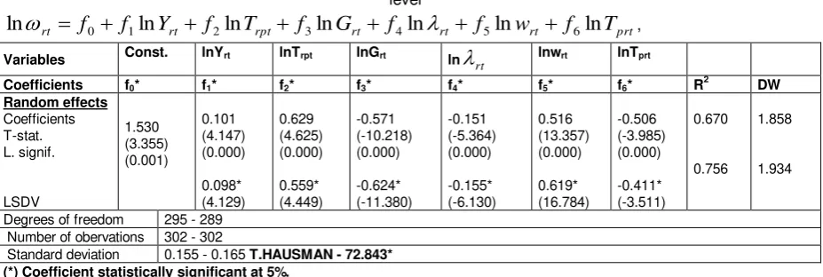
[image:5.595.69.533.501.657.2]

Table 4 presents the results of estimating equation 2 where the independent variables are disaggregated at regional level. About the signs of the coefficients, it appears that these are the expected, given the theory, the same can not be said of the variable



_rt (number of employees). However, it is not surprising given the economic characteristics of regions like the Norte (many employees and low wages) and Alentejo (few employees and high salaries), two atypical cases precisely for opposite reasons. Analyzing the results in Tables 2, 3 and 4 we confirm the greater explanatory power of the variables when considered in aggregate at the national level.

Table 4: Estimation of the equation of real wages with the independent variables disaggregated at the regional level

prt rt

rt rt

rpt rt

rt

f

ln

Y

f

ln

T

f

ln

G

f

ln

f

ln

w

f

ln

T

ln





₀



₁



₂



₃



₄





₅



₆ _,

Variables Const. lnYrt lnTrpt lnGrt _ln

rt



lnwrt lnTprt

Coefficients f0* f1* f2* f3* f4* f5* f6* R

2

DW Random effects

LSDV

1.530 (3.355) (0.001)

0.101 (4.147) (0.000)

0.098* (4.129)

0.629 (4.625) (0.000)

0.559* (4.449)

-0.571 (-10.218) (0.000)

-0.624* (-11.380)

-0.151 (-5.364) (0.000)

-0.155* (-6.130)

0.516 (13.357) (0.000)

0.619* (16.784)

-0.506 (-3.985) (0.000)

-0.411* (-3.511)

0.670

0.756

1.858

1.934

Degrees of freedom 295 - 289 Number of obervations 302 - 302

Standard deviation 0.155 - 0.165 T.HAUSMAN - 72.843* (*) Coefficient statistically significant at 5%.

7. ALTERNATIVE EQUATIONS TO THE EQUATIONS 1 AND 2

(6)

8. EQUATION OF THE AGGLOMERATION

In the analysis of the Portuguese regional agglomeration process, using models of New Economic Geography in the linear form, we pretend to identify whether there are between Portuguese regions, or not, forces of concentration of economic activity and population in one or a few regions (centripetal forces). These forces of attraction to this theory, are the differences that arise in real wages, since locations with higher real wages, have better conditions to begin the process of agglomeration. Therefore, it pretends to analyze the factors that originate convergence or divergence in real wages between Portuguese regions. Thus, given the characteristics of these regions will be used as the dependent variable, the ratio of real wages in each region and the region's leading real wages in this case (Lisboa e Vale do Tejo), following procedures of Armstrong (1995) and Dewhurst and Mutis-Gaitan (1995). So, which contribute to the increase in this ratio is a force that works against clutter (centrifugal force) and vice versa.

Thus:

rnt rkt

rgt rmt

rt nt

rl nt

lt rt

RL

a

RL

a

RL

a

RL

a

P

a

L

a

T

a

Y

a

ln

_



₀



₁



₂



₃



₄



₅



₆



₇



₈













(3)

where:

- Ynt is the national gross value added of each of the manufacturing industries considered in the database used; - Trl is the flow of goods from each region to Lisboa e Vale do Tejo, representing the transportation costs; - Lnt is the number of employees in manufacturing at the national level;

- Prt is the regional productivity (ratio of regional gross value added in manufacturing and the regional number of employees employed in this activity);

- RLrmt is the ratio between the total number of employees in regional manufacturing and the regional number of employees, in each manufacturing (agglomeration forces represent inter-industry, at regional level);

- RLrgt is the ratio between the number of regional employees in each manufacturing and regional total in all activities (represent agglomeration forces intra-industry, at regional level);

- RLrkt is the ratio between the number of regional employees in each manufacturing, and regional area (representing forces of agglomeration related to the size of the region);

- RLrnt is the ratio between the number of regional employees, in each of the manufacturing industries, and the national total in each industry (agglomeration forces represent inter-regions in each of the manufacturing industries considered).

The index r (1,..., 5) represents the respective region, t is the time period (8 years), n the entire national territory, k the area (km2), l the region Lisboa e Vale do Tejo, g all sectors and m manufacturing activity (9 industries).

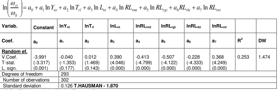
[image:6.595.68.532.558.709.2]

The results of the estimations made regarding equation 3 are shown in Tables 5 and 6. Two different estimates were made, one without the variable productivity (whose results are presented in Table 5) and one with this variable (Table 6).

Table 5: Estimation of the agglomeration equation without the productivity

rnt rkt

rgt rmt

nt rl

nt lt

rt

RL

a

RL

a

RL

a

RL

a

L

a

T

a

Y

a

ln

_



₀



₁



₂



₃



₄



₅



₆



₇













Variab. _{Constant lnY}nt lnTrl lnLnt lnRLrmt lnRLrgt lnRLrkt lnRLrnt

Coef. a0 a1 a2 a3 a4 a5 a6 a7 R2 DW

Random ef. V.Coef. T-stat. L. sign.

-3.991 (-3.317) (0.001)

-0.040 (-1.353) (0.177)

0.012 (1.469) (0.143)

0.390 (4.046) (0.000)

-0.413 (-4.799) (0.000)

-0.507 (-4.122) (0.000)

-0.228 (-4.333) (0.000)

0.368 (4.249) (0.000)

0.253 1.474

(7)

[image:7.595.67.530.118.305.2]

Table 6: Estimation of the agglomeration equation with the productivity rnt rkt rgt rmt rt nt rl nt lt

rt

_a

_ln

_Y

_a

_ln

_T

_a

_ln

_L

_a

_ln

_P

_a

_ln

_RL

_a

_ln

_RL

_a

_RL

_a

_ln

_RL

ln

8 7 6 5 4 3 2 1

0



















Variab. _{Constant lnY}nt lnTrl lnLnt lnPrt lnRLrmt lnRLrgt lnRLrkt lnRLrnt

Coef. a0* a1* a2* a3* a4* a5* a6* a7* a8* R

2 DW Random eff. V.Coef. T-stat. L. sign. LSDV -3.053 (-2.991) (0.003) -0.307* (-9.259) -0.240 (-7.182) (0.000) -0.033* (-4.821) 0.015 (2.026) (0.044) 0.330* (5.701) 0.486 (5.934) (0.000) 0.256* (8.874) 0.218 (8.850) (0.000) -0.049 (-0.972) -0.266 (-3.494) (0.001) 0.011 (0.169) -0.333 (-3.102) (0.002) -0.027 (-0.968) -0.141 (-3.067) (0.002) 0.006 (0.137) 0.230 (3.026) (0.003) 0.455 0.649 1.516 1.504

Degrees of freedom 292 - 285 Number of obervations 302 - 302

Standard deviation 0.116 - 0.136 T.HAUSMAN - 33.578* (*) Coefficient statistically significant at 5%.

Comparing the values of two tables is confirmed again the importance of productivity (Prt) in explaining the wage differences. On the other hand improves the statistical significance of coefficients and the degree of explanation.

9. EMPIRICAL EVIDENCE OF ABSOLUTE CONVERGENCE, PANEL DATA

Table 7 presents the results of absolute convergence of output per worker, obtained in the panel estimations for each of the economic sectors and the sectors to the total level of NUTS II, from 1986 to 1994 (a total of 45 observations, corresponding to regions 5 and 9 years).

[image:7.595.67.536.470.764.2]

The convergence results obtained in the estimations carried out are statistically satisfactory to each of the economic sectors and all sectors of the NUTS II.

Table 7: Analysis of convergence in productivity for each economic sectors of the five NUTS II of Portugal, for the period 1986 to 1994

Agriculture

Method Const. D1 D2 D3 D4 D5 Coef. T.C. DW R2 G.L.

Pooling 0.558 (1.200)

-0.063

(-1.163) -0.065 1.851 0.034 38

LSDV 4.127*

(4.119) 4.207* (4.116) 4.496* (4.121) 4.636* (4.159) 4.549* (4.091) -0.514*

(-4.108) -0.722 2.202 0.352 34

GLS 0.357 (0.915)

-0.040

(-0.871) -0.041 1.823 0.020 38 Industry

Pooling 2.906* (2.538)

-0.292*

(-2.525) -0.345 1.625 0.144 38

LSDV 6.404*

(4.345) 6.459* (4.344) 6.695* (4.341) 6.986* (4.369) 6.542* (4.334) -0.667*

(-4.344) -1.100 1.679 0.359 34

GLS 3.260* (2.741)

-0.328*

(-2.729) -0.397 1.613 0.164 38 Manufactured Industry

Pooling 1.806** (1.853)

-0.186**

(-1.845) -0.206 1.935 0.082 38

LSDV 6.625*

(4.304) 6.669* (4.303) 6.941* (4.303) 6.903* (4.318) 6.626* (4.293) -0.699*

(-4.301) -1.201 1.706 0.357 34

GLS 1.655** (1.753)

-0.171**

(-1.745) -0.188 1.946 0.074 38 Services

Pooling 5.405* (4.499)

-0.554*

(-4.477) -0.807 1.874 0.345 38

LSDV 7.193*

(5.290) 7.169* (5.301) 7.313* (5.284) 7.153* (5.292) 7.273* (5.293) -0.741*

(8)

GLS 5.627* (4.626)

-0.577*

(-4.604) -0.860 1.886 0.358 38 Services (without public sector)

Method Const. D1 D2 D3 D4 D5 Coef. T.C. DW R

2

G.L.

Pooling 5.865* (4.079)

-0.589*

(-4.073) -0.889 1.679 0.304 38

LSDV 6.526*

(4.197)

6.523* (4.195)

6.635* (4.191)

6.506* (4.176)

6.561* (4.192)

-0.658*

(-4.188) -1.073 1.684 0.342 34

GLS 5.027* (3.656)

-0.505*

(-3.649) -0.703 1.682 0.260 38 All sectors

Method Const. D1 D2 D3 D4 D5 Coef. T.C. DW R

2

G.L.

Pooling 3.166* (3.603)

-0.328*

(-3.558) -0.397 1.785 0.250 38

LSDV 6.080*

(5.361)

6.030* (5.374)

6.308* (5.347)

6.202* (5.379)

6.193* (5.359)

-0.643*

(-5.333) -1.030 2.181 0.460 34

GLS 3.655* (3.916)

-0.379*

(-3.874) -0.476 1.815 0.283 38 Note: Const. Constant; Coef., Coefficient, TC, annual rate of convergence; * Coefficient statistically significant at 5%, ** Coefficient statistically significant at 10%, GL, Degrees of freedom; LSDV, method of fixed effects with variables dummies; D1 ... D5, five variables dummies corresponding to five different regions, GLS, random effects method.

10. SOME FINAL CONCLUSIONS

In the estimates made for each of the economic sectors, with the Verdoorn law, it appears that the industry is the largest that has increasing returns to scale, followed by agriculture and service sector.

With the new economic geography models, it appears that the explanatory power of the independent variables considered, is more reasonable, when these variables are considered in their original form, in other words, in the aggregate form for all locations with strong business with that we are considering (in the case studied, aggregated at national level to mainland Portugal). On the other hand, given the existence of "backward and forward" linkages and agglomeration economies, represented in the variables Rlrmt and RLrgt, we can affirm the existence of growing scale economies in the Portuguese manufacturing industry during the period considered. It should be noted also that different estimates were made without the productivity variable and with this variable in order to be analyzed the importance of this variable in explaining the phenomenon of agglomeration. It seems important to carry out this analysis, because despite the economic theory consider the wages that can be explained by productivity, the new economic geography ignores it, at least explicitly, in their models, for reasons already mentioned widely, particular those related to the need to make the models tractable.

We find some signs of convergence, analyzing the results of the estimations with the models of the neoclassical theory.

So, for this period and for Portugal, the economic theory said that we have divergence between the continental regions, We have some signs of convergence, but is not enough to prevent the strong signs of divergence.

11. REFERENCES

1. N. Kaldor. Causes of the Slow Rate of Economics of the UK. An Inaugural Lecture. Cambridge: Cambridge University Press, 1966.

2. R.E. Rowthorn. What Remains of Kaldor Laws? Economic Journal, 85, 10-19 (1975).

3. M. Fujita; P. Krugman; and J.A. Venables. The Spatial Economy: Cities, Regions, and International Trade. MIT Press, Cambridge 2000.

4. F. Targetti and A.P. Thirlwall. The Essential Kaldor. Duckworth, London 1989.

5. P.J. Verdoorn. Fattori che Regolano lo Sviluppo Della Produttivita del Lavoro. L´Industria, 1, 3-10 (1949). 6. N. Islam. Growth Empirics : A Panel Data Approach. Quarterly Journal of Economics, 110, 1127-1170 (1995).

7. R. Solow. A Contribution to the Theory of Economic Growth. Quarterly Journal of Economics (1956).

8. V.J.P.D. Martinho. The Verdoorn law in the Portuguese regions: a panel data analysis. MPRA Paper 32186, University Library of Munich, Germany (2011a).

9. V.J.P.D. Martinho. Regional agglomeration in Portugal: a linear analysis. MPRA Paper 32337, University Library of Munich, Germany (2011b).

10. V.J.P.D. Martinho. Sectoral convergence in output per worker between Portuguese regions. MPRA Paper 32269, University Library of Munich, Germany (2011c).