An automatic procedure for the estimation of the tail index

Munich Personal RePEc Archive

An automatic procedure for the

estimation of the tail index

Gimeno, Ricardo and Gonzalez, Clara I.

2012

An Automatic Procedure for the Estimation of the

Tail Index

Ricardo Gimenoa,1_{, Clara I. Gonzalez}b,∗

a

Banco de España

b

FEDEA

Abstract

Extreme Value Theory is increasingly used in the modelling of financial time

series. The non-normality of stock returns leads to the search for alternative

distributions that allows skewness and leptokurtic behavior. One of the most

used distributions is the Pareto Distribution because it allows non-normal

behaviour, which requires the estimation of a tail index.

This paper provides a new method for estimating the tail index. We

propose an automatic procedure based on the computation of successive

nor-mality tests over the whole of the distribution in order to estimate a Gaussian

Distribution for the central returns and two Pareto distributions for the tails.

We find that the method proposed is an automatic procedure that can be

computed without need of an external agent to take the decision, so it is

clearly objective.

Keywords: Tail Index; Hill estimator; Normality Test

∗_{Corresponding author. Foundation for Applied Economic Studies (FEDEA). Jorge}

Juan 46, 28001 Madrid (Spain). e-mail: [email protected]

1. Introduction

Extreme price movements are a common fact during the normal

function-ing of financial markets and durfunction-ing highly volatile periods correspondfunction-ing to

financial crises, like for example stock market crashes.

In the last decades, researches has been focused in modelling and

esti-mating financial time series. However, most of this studies are concerned

about expected returns, volatility or correlations, and not so much attention

has been paid to extreme movements. Previous works in the use of extreme

value to explain the fluctuations of the financial time series are Rothschild

and Stiglitz (1970), who used the weight of the tails of two random

vari-ables in order to suggest a best definition of the risk increase than the usual

variance, Parkinson (1980) discovered that extreme values offer an useful

in-formation in order to estimate volatility more efficiently, Haan et al. (1989)

showed that the maximum of a distribution will be a Frechet one if the change

in the stock price follows an ARCH process, Jansen and de Vries (1991) used

extreme values in order to research the fat of the distribution tails.

It is a common conclusion in financial literature that the distribution of

stock returns shows heavy tails, it means that there are more realizations in

the tails than is to be expected if it had a normal distribution. In other words,

stock return data shows more extreme realizations than can be accounted for

by the normal distribution. Moreover round the mean value, the very small

movements, there are more likelihood than expected. So the medium values

are going to show a lower likelihood than the normal behavior. Originally

Mandelbrot (1963), and later Fama (1965), pointed out that the distribution

which implies that it is peaked and fat-tailed.

This observation is of vital importance to risk management, and in

par-ticular to Value-at-Risk analysis, because it is the behavior of extremely

low returns that causes large losses. EVT is a useful supplementary risk

measure in risk management as a method for modelling and measuring this

extreme risks. The seminal work of EVT is the one of Gnedenko (1943)

who establishes three types of non-degenerated distributions for the

stan-dardized maximum: Frechet, Weibull and Gumbel. Galambos (1978) gives a

rigorous account of the probability aspects of extreme value theory. Longin

(1996) analysis extreme movements in the U.S. stock market, and obtains

empirically that the extreme returns has a Frechet distribution. Moreover,

applications of extreme value theory in insurance and finance can be found

in Embrechts et al. (1997) and Reiss and Thomas (1997).

The structure of this article is as follows, in section 2 Extreme Value

The-ory is introduced. Then we brought up the Generalized Pareto Distribution

in section 3 and the Pareto Distribution in section 4. Finally, in section 5 is

proposed a new methodology for the estimation of the threshold value of the

tail index.

2. Introduction to Extreme Value Theory

There are two classes of extreme value distributions who are used to find

the correct limit distributions for maxima and minima. The first class was

proposed by Jenkinson (1955), a Generalized Extreme Value (GEV)

distribu-tion that includes the three standard extreme value distribudistribu-tions established

The second class includes the distribution of excess over a given threshold,

what it is interesting in modelling the behavior of the excess loss once a

high threshold (loss) is reached. A more modern group of models are the

Peaks-Over-Threshold (POT) models, that can be used to estimate the excess

distribution with respect to a threshold levela, and to estimate the tail shape

of the original distribution.

Within the POT class of models we can find two sorts of models, one

of them is the semi-parametric model family built around the Hill estimator

and its relatives Beirlant et al. (1996); Danielsson et al. (1998) and other are

the fully parametric models based on de generalized Pareto distribution or

GDP Embrechts et al. (1999).

There has been in the last years several researches about the adaptation

of the stable Pareto distribution in order to model the unconditional

dis-tribution of returns, the first considerations about it are the researches of

Mandelbrot (1963) and Fama (1963, 1965). Not always the stable class of

models are suitable to apply to leptokurtic and skewed returns, despite they

are suitable in a theoretical approach.

Hill estimator (Hill, 1975) and other similar tail estimators, are known

because they are not reliable in-even large-finite samples (cf. Mittnik and

Rachev (1993), McCulloch (1997), Resnick (1997) and Mittnik et al. (1998))

3. Generalized Pareto Distribution

The Generalised Pareto Distribution (GPD) is a two parameter

distribu-tion and its importance in extreme value theory was observed by Pickands

(1975) who showed basically that the GDP offers a good approximation of

the tail of the distribution of returns for some fixed ξ as a shape parameter

and β as an additional parameter that is β > 0. Its distribution function is

the following,

Gξ,β(x) =   

1−1 +ξX β

−1

ξ

if ξ 6= 0

1−e−Xβ if ξ = 0

 

 (1)

where x≥0when ξ≥0and 0≤x≤ −β

ξ whenξ < 0. The sign of the shape

parameter ξ determines its tail behavior and thus the tail behavior of the

original distribution.

This distribution is generalized in the sense that it subsumes other

dis-tributions under a common parametric form. If ξ > 0 the tail of the

distri-bution function Gξ,β(x) decays like a power function x−

1

ξ, in this case, the

function Gξ,β belongs to a family of heavy-tailed distributions that includes:

the Pareto, log-gamma, Cauchy and t-distributions and others. Forξ = 0the

tail forGξ,β decreases exponentially, and belongs to a class of medium-tailed

distributions that include the normal, exponential, gamma and lognormal

distributions. Finally if, ξ <0is known as a Pareto Type II distribution, the

underlying distribution Gξ,β is characterized by a finite right endpoint, this

4. The Pareto Distribution

The first of the three previous groups of distributions, when ξ > 0, is

the most relevant case for risk management purposes because implies a GDP

with heavy tails. This is the reason why the Pareto distribution is the most

used in fat-tailed distributions. It is considered as a truncated distribution,

because the right tail of the distribution has values greater than an specific

value a or threshold. It has this probability density distribution

f(x, a, α) = α a

α

xα+1 (2)

with x≥a and α the tail index.

But we are interested in the extreme movements that lead to large losses,

so we have to focus on the left tail where the values are below a certain

thresh-old level. The cumulative distribution function of the Pareto distribution will

be

F(−x)≈ax−α ₍₃₎

with α >0.

The issue is how we can obtain the value of a or threshold level and

of α or tail index, if the threshold is known then α can be estimated by

the maximum likelihood method. The maximum likelihood estimator of the

reciprocal of the tail index, γ ≡ 1/α, is obtained from the Hill estimator

(Hill, 1975): (equation 4),

b

γH ≡1/αbM L = n X

i=1

log xi a

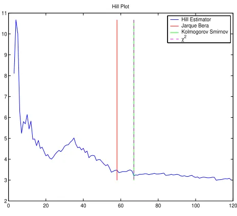
We usually not know the threshold valuea from where the empirical

dis-tribution behaves as a Pareto disdis-tribution, the choice off this cut-off point is

the more important of all the estimation results. In order to find it, the usual

method consists in calculating and plotting the Hill estimator for different

values of the threshold a (Drees et al., 2000), to search those value where

the tail index is stable, so that the threshold a is selected from the hill plot

for the stable areas of the tail index (In figure 1 we present the Hill plot for

the FTSE 100 index). However, this choice is not always clear. In fact, this

method applies well for a GPD or close to GPD type distribution. As stated

by Bensalah (2000), the Hill estimator is the maximum likelihood for a GPD

and since the extreme distribution converges to a GPD over a high threshold

u its use is justified.

5. The distribution of financial returns. Identification of outliers

It is a common place now in the literature, since the initial works of

Mandelbrot (1963) and Fama (1965) that the hypothesis of normality must

be rejected. The three features that are commonly alleged as the causes of

this rejection are:

1. Fat tails or extreme values in the distribution. The tails of the

distri-butions concentrate more probability than is supposed on a Gaussian

distribution.

2. Cluster of probability near the mean value of the distribution. Most of

the movements in asset prices are relatively small.

3. The extreme movements are more frequent in the left side of the

news.

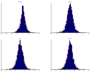
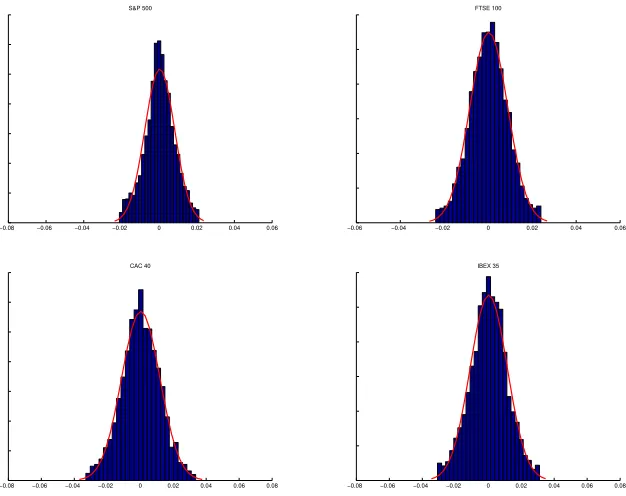
The first two features lead to a leptokurtic distribution, and the third

feature to the presence of skewness in the distribution. Figure 2 shows this

features plotting the histogram of the returns in the case of four different

stock indexes: S&P500 (NYSE), FTSE100 (London), CAC40 (Paris) and

IBEX35 (Madrid). Table 1 shows the mean, standard deviation, skewness

(g3 = m

3

s3) and kurtosis (g4 = m

4

s4 −3) coefficient. All of them have left

skewness and an excess of kurtosis.

Extreme Value Theory as it is applied to financial markets assume that

the tails of the distribution are governed by a different function than the rest

of the distribution. The tails are then fitted with a Pareto distribution as

presented in section 4. The Hill estimator (equation 4) is then used to split

the returns in extreme and non-extreme returns. This estimation explains

one of the three features of the asset returns and require a subjective selection

of the threshold in the region where the hill estimator remains stable (Figure

1).

It is our aim to obtain a method for the estimation of the threshold that

not only explains the fat tails, but also the skewness and kurtosis of the

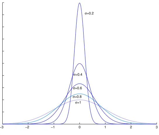
distribution. The distribution of the whole asset returns can be obtained as

a mixture of a gaussian function for the center of the distribution and two

Pareto laws for both tails as presented in figure 3.

If the tails are explained by two Pareto laws, the rest of the distribution

will have a lower standard deviation. After diminishing the value of the

variance, the gaussian function will be concentrated around the mean value

laws would explain not only the fat tails but the cluster on the mean value

and even the skewness if we consider a different Pareto law for each tail.

We propose to fit the lower price movements to a normal distribution

instead of trying to fit the tails of the distribution. Our proposal is to identify

the asset returns that cannot be considered gaussian, and will be treated as

outliers that we will be modelled by a Pareto distribution.

Given a time series of asset returns,xi, the process of identification of the

values from both distribution will be as follows:

1. We define the absolute returns, yi=|xi| ∀i= 1, . . . , T. A higher value

will imply a strong movement of the asset price, doesn’t matter if it is

positive or negative.

2. We order the values of yj, such as y1 ≥ y2 ≥ y3 ≥ . . . ≥ yT, and save

the ordination index.

3. We test the normality hypothesis for the subset {xj}∀j =r, . . . , T.

4. We select the value of r that produce a better result in the normality

test.

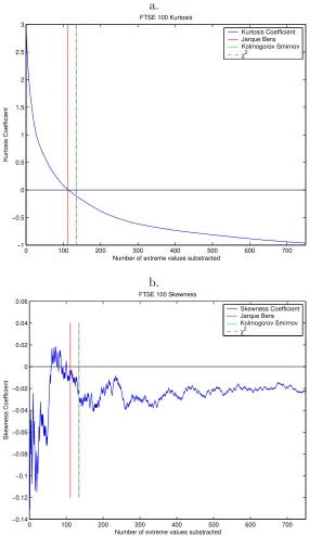
As we eliminate the extremal values we reduce the excess of kurtosis.

The kurtosis coefficient for the returns of the FTSE 100 index is plotted in

figure 5a. After eliminating a sufficient number of extreme value we pass

from a leptokurtic to a platykurtic distribution. But also the skewness of the

distribution (figure 5b) is reduced in the process. In Figure 6 can be seen

the resulting distributions for the four indexes.

In order to test the normality of the distribution we have chosen three

1. χ2

goodness of fit. Also known as test χ2

, this test present as null

hypothesis that the sample has been obtained from a variable with

probability distribution equal to P, i.e. the normal distribution.

We will have a sample called X with observations that could be

classi-fied inrclasses (i.e. the intervals of an histogram). We could represent

this categories by A1, A2, . . . , Ar. In the sample X there are n1

ele-ments that belongs to category A1, n2 elements that belongs to A2

and so on. Under the null hypothesis, we know the probability of each

class, P(Ai) = pi, where p1 +p2 +. . .+pr = 1. The probability of

obtaining n1, n2, . . . , nr elements of each class will have a multinomial

distribution with probabilities,

P(n1, n2, . . . , nr) =

n! n1!· · ·nr

pn1

1 · · ·p

nr

r (5)

where each ni has a marginal binomial distribution B(n, pi) with an

expected value, E(ni) = npi = Ei. This expected value called Ei

represents the number of observations belonging to class Ai, that we

expect if the null hypothesis is true. So we construct an statistic,

r X

i=1

(ni −Ei)

Ei

χ2

r−k−1 (6)

under the null hypothesis, where k is the number of parameters

esti-mated on the null hypothesis distribution (i.e. µ and σ in the case of

a normal distribution)

For a continuous distribution we obtain the classes and the ni

val-ues from an histogram, and the correspondent pi from the expression

order to obtain not-empty intervals we select the extremesxi that have

equal values of ni.

2. Kolmogorov Smirnov test. It compares the values of the theorized

normal distribution function and the empirical sample distribution.

The test compute the maximum difference between both distributions

(equation 7).

D= sup

x

|Ft(x)−Fr(x)| (7)

3. Jarque Bera test (Jarque and Bera, 1980). It is based on the kurtosis

and skewness coefficients, comparing the results of both coefficients in

the sample with the values of a gaussian distribution (equation 8).

JB = T −k 6 m3 s3 2 + m4 s4 −3 2 1 4 !

∼χ2

2 (8)

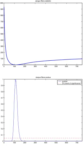
In figure 7 it is possible to see how as we eliminate the extreme values of

the sample, the Jarque-Bera test gives increasing values, reaching a threshold

in which the test accept the null hypothesis of normality. Figure 7 implies

that for the FTSE 100 index it is possible to reach a pvalue of 0.999 in the

Jarque-Bera test. If we continue eliminating values we pass from a problem

from the leptokurtic shape of the distribution to the opposite problem of

platykurtic distribution. This is clear if we observe figure 5 where the kurtosis

and skewness of the distribution is presented against the number of extremal

returns subtracted. In the same figure 5 it is possible to see the value of the

threshold a for the three normality tests used. Jarque-Bera select a value

that gives skewness and kurtosis coefficients closer to the ones expected in a

6. Conclusions

Fama (1963) and Mandelbrot (1965) proved empirically that stock returns

do not have a Gaussian Distribution so it is necessary to select an alternative

distribution that allows skewness and leptokurtic behaviour. The Extreme

Value Theory is increasingly used in the modelling of financial time series

and the Pareto Distribution is one of the most widely used because it allows

non-normal behaviour.

The estimation of the tail index is usually obtained by plotting the Hill

Estimator for different values of the threshold, choosing that value where

this estimator becomes stable. However, this procedure requires a subjective

choice on the part of the researcher and in addition it is not automatic.

This paper provides a new method for estimating the tail index of the

distribution of stock returns.In this paper, successive normality tests are

realized over the whole of the distribution in order to estimate a Gaussian

Distribution for the central returns and two Pareto distributions for the tails.

It is possible to see that the threshold estimations obtained by the

nor-mality tests lies in the plateau of the Hill plot (figure 1). These threshold

estimators are consistent with the results obtained with the Hill plot, but

with the great advantage of been an automatic procedure that can be

References

Beirlant, J., Teugels, J., Vynckier, P., 1996. Practical analysis of extreme

values. Tech. rep., Leuven University Press, Leuven.

Bensalah, Y., 2000. Steps in applying extreme value theory to finance: A

review. Working Paper 20, Bank of Canada.

Danielsson, J., Hartmann, P., de Vries, C. G., January 1998. The cost of

conservatism: Extreme returns, value-at-risk, and the basle multiplication

factor. Risk.

Drees, H., de Haan, L., Resnick, S., 2000. How to make a hill plot. The

Annals of Statistics 28, 254–274.

Embrechts, P., Klüppelberg, C., Mikosch, T., 1997. Modelling Extremal

Events. Springer Verlag, Berlin.

Embrechts, P., Resnick, S., Samorodnitsky, G., 1999. Extreme value theory

as a risk management tool. North American Actuarial Journal 3, 30–41.

Fama, E. F., 1963. Mandelbrot and the stable paretian hypothesis. Journal

of Business 36 (4), 420–429.

Fama, E. F., 1965. The behavior of stock market prices. Journal of Business

38, 34–105.

Galambos, J., 1978. The Asymptotic Theory of Extreme Order Statistics.

Gnedenko, B., 1943. Sur la distribution limite du terme maximum d’une serie

aleatoire. Annals of Mathematics 44, 423–453.

Haan, L. D., Resnick, I. S., Rootzen, H., de Vries, C., 1989. Extremal

be-havior of solutions to a stochastic difference equation with applications to

arch process. Stochastic Processes and Their Applications 32, 213–224.

Hill, B., 1975. A simple general approach to inference about the tail of a

distribution. Annals of Statistics 3, 1163–1174.

Jansen, D., de Vries, C., 1991. On the frequency of large stock returns:

putting booms and busts into perspective. Review of Economics and

Statis-tics 73, 18–24.

Jarque, C. M., Bera, A. K., 1980. Efficient tests for normality,

homoscedastic-ity and serial independence of regression residuals. Economics Letters (6),

255–259.

Jenkinson, A., 1955. The frequency distribution of the annual maximum

(or minimum) values of meteorological elements. Quarterly Journal of the

Royal Meteorological Society 87, 145–158.

Longin, F., 1996. The asymptotic distribution of extreme stock market

re-turns. Journal of Business 69, 383–408.

Mandelbrot, B., 1963. The variation of certain speculative prices. Journal of

Business 36, 394–419.

index alpha: A critique. Journal of Business & Economic Statistics 15 (1),

74–81.

Mittnik, S., Paolella, M., Rachev, S., 1998. A tail estimator for the index of

the stable paretian distribution. Communications in Statistics Theory and

Methods 27 (5), 1239–1262.

Mittnik, S., Paolella, M. S., Rachev, S. T., 2000. Diagnosing and treating

the fat tails in financial returns data. Journal of Empirical Finance (7),

389–416.

Mittnik, S., Rachev, S., 1993. Modeling asset returns with alternative stable

models. Econometric Reviews 12, 261–330.

Parkinson, M., 1980. The extreme value method for estimating the variance

of the rate of returns. Journal of Business 53, 61–65.

Pickands, J., 1975. Statistical inference using extreme order statistics. Annals

of Statistics 3, 119–131.

Reiss, R., Thomas, M., 1997. Statistical Analysis of Extreme Values.

Birkhäuser, Basel.

Resnick, S., 1997. Heavy tail modeling and teletraffic data. Annals of

Statis-tics 25 (5), 1805–1869.

Rothschild, M., Stiglitz, J. E., 1970. Increasing risk: I. a definition. Journal

0 20 40 60 80 100 120 2

3 4 5 6 7 8 9 10 11

Hill Plot

Hill Estimator Jarque Bera Kolmogorov Smirnov

χ2

Figure 1: Hill plot of the FTSE 100 index and the values of the tail threshold with the

−0.08 −0.06 −0.04 −0.02 0 0.02 0.04 0.06 S&P 500

−0.06 −0.04 −0.02 0 0.02 0.04 0.06 FTSE 100

−0.08 −0.06 −0.04 −0.02 0 0.02 0.04 0.06 0.08 CAC 40

−0.08 −0.06 −0.04 −0.02 0 0.02 0.04 0.06 0.08 IBEX 35

Figure 2: Histogram of the returns of the indexes S&P 500, FTSE 100, CAC 40 and IBEX

Gaussian Distribution Rigth Pareto Distribution Left Pareto Distribution

−3 −2 −1 0 1 2 3 σ=1

σ=0.8 σ=0.6 σ=0.4

σ=0.2

Table 1: Descriptive statistics from four stock index daily returns(S&P 500, FTSE 100,

CAC 40, IBEX 35)

Mean Std. Deviation Skewness kurtosis

S&P 500 0,000284268 0,010479535 -0,123687694 3,922177894

FTSE 100 0,000164333 0,01055061 -0,130502363 2,8471159

CAC 40 0,000147307 0,013697291 -0,1205063 2,544084239

IBEX 35 0,000214679 0,013742123 -0,145496279 2,757789877

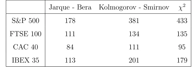
Table 2: Number of observation subtracted in each index according with the gaussian test

used

Jarque - Bera Kolmogorov - Smirnov χ2

S&P 500 178 381 433

FTSE 100 111 134 135

CAC 40 84 111 95

a.

0 100 200 300 400 500 600 700

−1 −0.5 0 0.5 1 1.5 2 2.5 3

FTSE 100 Kurtosis

Kurtosis Coefficient

Number of extreme values substracted

Kurtosis Coefficient Jarque Bera Kolmogorov Smirnov χ2

b.

0 100 200 300 400 500 600 700

−0.14 −0.12 −0.1 −0.08 −0.06 −0.04 −0.02 0 0.02 0.04 0.06

FTSE 100 Skewness

Skewness Coefficient

Number of extreme values substracted

Skewness Coefficient Jarque Bera Kolmogorov Smirnov χ2

Figure 5: Returns of FTSE 100 (a. Skewness Coefficient and b. kurtosis Coefficient). In

−0.08 −0.06 −0.04 −0.02 0 0.02 0.04 0.06 S&P 500

−0.06 −0.04 −0.02 0 0.02 0.04 0.06 FTSE 100

−0.08 −0.06 −0.04 −0.02 0 0.02 0.04 0.06 0.08 CAC 40

−0.08 −0.06 −0.04 −0.02 0 0.02 0.04 0.06 0.08 IBEX 35

Figure 6: Histogram of the returns of the indexes S&P 500, FTSE 100, CAC 40 and IBEX

0 100 200 300 400 500 600 700 0

100 200 300 400 500 600 700 800 900 1000

Jarque Bera statistic

0 100 200 300 400 500 600 700

0 0.1 0.2 0.3 0.4 0.5 0.6 0.7 0.8 0.9 1

Jarque Bera pvalue

pvalue

5% level of significance

Figure 7: Jarque Bera test on the returns of FTSE 100 (a. Jarque-Bera test b. P-value).