Forecasting Performance of Alternative Error Correction Models

Munich Personal RePEc Archive

Forecasting Performance of Alternative

Error Correction Models

Iqbal, Javed

Karachi University

19 March 2011

Online at

https://mpra.ub.uni-muenchen.de/29826/

Forecasting Performance of Alternative Error Correction Models

By Javed Iqbal Department of Statistics

Karachi University Karachi Pakistan

Email: [email protected]

Preliminary draft: Not for publication

Abstract

Forecasting Performance of Alternative Error Correction Models

It is well established that regression analysis on non-stationary time series data may yield

spurious results. An earlier response to this problem was to run regression with first

difference of variables. But this transformation destroys any long-run information

embodied in the levels of variables. According to ‘Granger Representation Theorem’

(Engle and Granger, 1987) if variables are co-integrated, there exist an error correction

mechanism which incorporates long run information in modeling changes in variables.

This mechanism employs an additional lag value of the disequilibrium error as an

additional variable in modeling changes in variables. It has been argued that ECM

performs better for long run forecast than a simple first difference or level regression.

This process contributes to the literature in two important ways. Firstly empirical

evidence does not exist on the relative merits of ECM arrived at using alternative

co-integration techniques. The three popular co-co-integration procedures considered are the

Engle-Granger (1987) two step procedure, the Johansen (1988) multivariate system based

technique and the recently developed Autoregressive Distributed Lag based technique of

Pesaran et al. (1996, 2001). Secondly, earlier studies on the forecasting performance of

the ECM employed macroeconomic data on developed economies i.e. the US and the

UK. By employing data form the Asian countries and using absolute version of the

purchasing power parity and money demand function this paper compares forecast

accuracy of the three alternative error correction models in forecasting the nominal

1. Introduction:

The Granger Representation Theorem (Engle and Granger, 1987) enables simultaneous

modeling of first difference and the levels of the variables using an error correction

mechanism which provides the framework for estimation, forecasting and testing of

co-integrated systems. If Xtand Ytare individually I(1) variables are co-integrated with

cointegration vector (1,0,1)the general form of the ECM can be expressed as

t t t

t

t B L X Y X u

Y L

A( )   ( ) ( _10 1 _1) (1)

with the lag polynomials

p pL a L a L a L

A( )1  2 ...

2 1 ; q qL b L b L b b L

B( )   2...

2 1

0

where the lag operator is defined as t t i i

Y Y

L  _ . In this model the coefficients in the A(L)

and B(L) represent the impact of short changes while the long run effects are given by

the co-integration vector (1,0,1) and the  controls the speed of adjustment short

run changes towards long run path.

As co-integration and ECM provides a unified framework of molding both long and short

run an interesting question for researcher was whether incorporating the long-run

restriction in an error correction models yields superiors forecast in comparison with pure

first difference models which do not impose co-integration restrictions. On a theoretical

ground co-integration is expected to yield better forecast as pointed by Stock (1995, p-1)

who asserts that “If variables are co-integrated, their values are linked over the long run,

and imposing this information can produce substantial improvements in forecast over

that long horizon forecasts from the co-integrated systems satisfy the co-integration

relationship exactly and that the cointegration combination of variables can be forecast

with finite long-horizon forecast error variance.

A simulation study by Engle and Yoo (1987) shows that the two step EG ECM provide

better forecast compared to unrestricted VAR particularly at longer horizons while the

similar simulation study by Chambers(1993) further corroborated this result using a

non-linear one-step ECM. Using the same experimental set up as Engle and Yoo, Clements

and Hendry (1995) find that over-differencing the system results in inferior forecasting

performance. In a simulation study using a four-dimensional VAR(2) Reinsel and Ahn

(1992) show that forecast gains from co-integrated system depends on proper

specification of the number of unit roots and under specifying the number of unit roots

results in poor performance for ten to twenty five steps ahead forecasts whereas

over-specification results in inferior short-term forecasts

After the pioneering two-step estimator of the ECM parameters proposed by Engle and

Granger (1987) several ECM techniques have been developed. The Engle-Granger

technique can identify only a single equilibrium relationship among the variables under

study. Johansen (1988) proposed a frame work of estimation and testing of vector error

correction model (VECM) based on vector auto regression (VAR) equations. The VECM

can be expressed as:



 

   

 

 p

j

t j t j t

t Y Y u

Y

1

The is an mm matrix containing the long-run parameters. If there are r

co-integration vectors then can be expressed as a product of tow matrices as'wher

both  and  are mrmatrices. The matrix contains the coefficients of long-run

relationship and the  contains the speed of adjustment parameters which is also

interpreted as the weight with which each co-integration vectors appears in a given

equation.

This approach can accommodate multiple equilibrium relationships in the VECM. Both

of these estimation techniques assume that the variables to be modeled are I(1). Recently

Pesaran, Shin and Smith (1996) and Pesarn (2001) proposed a techniques based on

Autoregressive Distributed Lag (ARDL) model which allows both I(0) and I(1) variables

thus potentially avoids pre-test bias. In the literature some studies have compared forecast

ability of the ECM resulting from the Engle-Granger and the Johansen VECM technique.

However the literature does not provide empirical evidence regarding the forecast

accuracy of the ARDL based ECM and its comparison with EG and Johansen techniques.

In addition, most of the empirical evidence employing real data in forecast comparison

comes from the developed economies. This study provides empirical evidence of

forecasting performance of the ECM resulting from the three techniques from Asian

countries.

2. The Literature

Hoffman and Rasche (1996) compared the forecast performance of a cointegrated system

relative to the forecast performance of a comparable VAR that fails to recognize that the

system is characterized by cointegration. They considered cointegrated system

premium captured by an interest rate differential. The data were from the US economy.

They found that the advantage in imposing co-ingratiation appears only at loner forecast

horizon and this is also sensitive to the appropriate data transformation. They considered

8 years out-sample forecast horizon.

Jansen and Wang (2006) investigated the forecasting performance of the Error Correction

model arising from the co-integrating relationship between the equity yield on the S&P

500 and the bond yield relative to that of univariate models. They found that the Fed

Model improves on the univariate model for longer-horizon forecasts, and the nonlinear

vector error correction model performs even better than its linear version. The forecast

horizon they considered was 10 years.

Wang and Bessler (2004) employed five US agriculture time series. They used annual

data from 1867 to 1966 for model specification and data for 1966 to 2000 were used for

out-of sample forecast evaluation. Their results favored ECM for three to four steps

ahead forecasts. However the differences in forecast obtained from different models were

not statistically significant.

Lin and Tsay (1996) considered both simulated and financial and macroeconomic real

data from the UK, Canada, Germany, France and Japan and interest rate data from the

US and Taiwan. Their results are contradictory as the simulated data yield better forecast

fro the ECM whereas for real data the performance of ECM is mixed. They attribute this

contradiction to deficiency in forecast error measure which does not recognize that

forecast are tied together in the long-run.

This brief literature review indicates that at best the results on relative merit of imposing

longer horizon. An important observation from this review is that very few studies

employ data from the less developed economies such as East and South Asian economies.

Also no study has yet considered forecasting performance of the newly developed ARDL

based co-integration. It has been argued that ARDL has important advantages over the

Engle-Granger and Johansen approaches. Firstly it can be applied irrespective of whether

underlying repressors are I(0) or I(1). Secondly in simulation studies it performs better

than EG and Johansen co-integration test in small samples. Thirdly appropriate

modification of the orders of the ARDL model is sufficient to simultaneously correct for

residual serial correlation and the problem of endogenous variables.

3.The data and the models

The economic models we considered are the Purchasing Power Parity and the money

demand function. The absolute PPP states that exchange rate between two currencies

adjust to remove any arbitrage opportunities (buy in a low price market and sell with a

profit in a high price market). If PPP holds then in the long run exchange rate equals ratio

of prices in the two economies. i.e. the intercept equals zero and slope equals 1 in the

equation:log(e)t 01log(CPIRatio)t ut (3)

Secondly we considered demand of real money balances depends positively on

transaction volume (output level) and negatively on cost of holding cash i.e. interest rate

i.e.

t t t

t Y R u

CPI

M / )  ₀  ₁log( )  ₂ 

Thus the task is to forecast exchange rate (local currency per dollar) and money stock

(M2) from the alternative ECM resulting from the three co-integration techniques. The

quarterly data (1978Q1-2009Q4) of ten Asian countries are employed namely

1. Korea 2. Singapore 3. Malaysia 4. Indonesia 5. Thailand 6. Philippines 7. Sri Lanka 8.

India 9. Pakistan 10. Bangladesh.

Interest rate is measured by discount rate, lending rate or money market rate (whichever

is available for full sample period) Output is measured by manufacturing production

index which indicate significant seasonality so quarterly dummies are added in

estimation. The data comes mostly from IFS. Thai manufacturing production index is

obtained from Bank of Thailand. The output data for Sri Lanka are not available so

money demand results are not presented for Sri Lanka.

In the empirical analysis possess certain challenges e.g. EG and Johansen require the

pre-testing for unit root in the variables and strictly speaking are valid if variables are I(1).

However ARDL does not need such pre-testing. Unit root tests on all the series were

conducted using ADF, Phillips-Perron and KPSS methods. In some cases EG, Johansen

and ARDL co-integration tests could not uncover any co-integration however in most

cases the co-integration evidence comes from significance of Error Correction term. The

analysis is conducted for all countries despite these limitations.

We considered quarterly data from 1978Q1 to 2009Q4. For model specification and

estimation we employ data from 1978Q1 to 1994Q4 and the forecast evaluation is

conducted from the period 2005Q1 and 2009Q4. We employ Mean Absolute Percentage

scaling of variables so that forecast error from countries is comparable MAPE is given

by:



    H t t t t Y Y Y H MAPE 1 | ˆ | 1 100

Where Ytand Yˆt represent actual and forecast respectively.

5. Results and Discussion

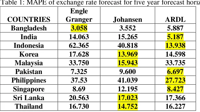
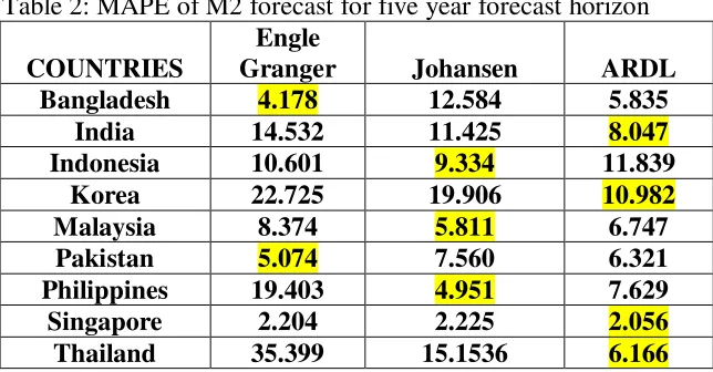
The following tables (Table 1 and Table 2) present the comparison of forecast accuracy

based on MAPE. The best ECM model in each case is highlighted. Generally the ARDL

appears to yield lower forecast errors followed by Johansen technique. This is the case

for money stock forecast (Table 2) where potentially more than one co-integration

vectors are possible. For Bangladesh the EG ECM yields the best forecast for the two

variables. For Malaysia Johansen technique appears to be superior. For India and

Singapore the ARDL technique results in the lowest forecast error. The results for other

countries are mixed for the two variables.

Table 1: MAPE of exchange rate forecast for five year forecast horizon

COUNTRIES

Engle

Granger Johansen ARDL

Bangladesh 3.058 3.552 5.887

India 14.063 15.265 5.187

Indonesia 62.365 40.818 13.938

Korea 17.628 13.969 14.598

Malaysia 33.750 15.943 33.735

Pakistan 7.325 9.600 6.697

Philippines 37.53 41.039 27.723

Singapore 8.69 12.195 8.427

Sri Lanka 20.563 17.023 17.366

Thailand 16.730 14.752 16.227

Notes: Schwarz criteria selects lag 1 as optimal for Engle-Granger method for all ten countries. Regression of ECM model with this optimal lags indicate that error correction term is insignificant only in Sri Lanka.

was insignificant only in Indonesia. In other cases loading coefficient was significant with negative sign in at least one VECM equation.

Optimal lags using Schwarz criteria for ARDL is 1 for all countries. With optimal lags ECT term is insignificant only in Indonesia.

Table 2: MAPE of M2 forecast for five year forecast horizon

COUNTRIES

Engle

Granger Johansen ARDL

Bangladesh 4.178 12.584 5.835

India 14.532 11.425 8.047

Indonesia 10.601 9.334 11.839

Korea 22.725 19.906 10.982

Malaysia 8.374 5.811 6.747

Pakistan 5.074 7.560 6.321

Philippines 19.403 4.951 7.629

Singapore 2.204 2.225 2.056

Thailand 35.399 15.1536 6.166

Notes: Optimal lags for Engle-Granger test are 1 for all counties. In some countries Engle-Granger ADF test did not uncover co-integration but subsequent in ECM model error correction term is insignificant only in Korea, Malaysia and Pakistan.

Optimal lags for Johansen vary over different countries using same lags for each variable. Trace and Max statistics do not indicate co-integration but in VECM models the loading coefficients was insignificant only in Indonesia.

Optimal lags using Schwarz criteria using ARDL method are four for Korea, Philippines, Pakistan and Bangladesh; three for Singapore and one for India, Malaysia, Thailand. With optimal lags error correction term is insignificant only in Malaysia and Pakistan

Manufacturing production for Sri Lanka is not available so money demand estimation is not possible.

6. Conclusion

It is well known that regression analysis on non-stationary time series data may be

spurious (non-sense) if the underlying variables are not co-integrated. Error correction

models provide a convenient solution for estimation, testing and forecasting. However

there are now different co-integration estimation and testing techniques have been

developed. In this paper we have compared the forecast accuracy of three popular error

correction models that are derived from the Engle-Granger, Johansen and the ARDL

techniques. The results indicate that in general the ECM based on both the ARDL and

in the best performance in about 48% of the cases whereas the Johansen’s ECM yields

the best performance in about 36% cases. The ARDL technique appears to be superior

even in cases where more than one co-integration relationships are possible i.e. money

demand model which involve three variables in the system. The average MAPE for

exchange rate forecast across ten countries is 15%, 18.4% and 22.5% for the ARDL,

Johansen and the EG techniques respectively. The average MAPE for M2 forecasts are

7.3%, 9.9% and 13.6% for the ARDL, Johansen and the EG techniques respectively.

Thus our analysis provides evidence in favor of the ARDL based ECM. Also it will be

interesting to compare forecast of ECM from alternative techniques which do not impose

References

Chambers , M.J. (1993). A note on forecasting in co-integrated systems. Computers

Method Application s, 25, 93-99.

Clements, M. P. and D. F. Hendry (1995), Forecasting in co-integrated systems. Journal

of Applied Econometrics10, 127-146.

Engle, R.F. and Granger, C.W.J. (1987).Co-integration and error correction:

Representation, estimation and testing, Econometrica 55,251-276

Engle, R.F. and Yoo, B.S. (1987). Forecasting and testing in co-integrated systems, the

Journal of Econometrics, 35,143-159.

Haigh, M.S. (2000). Co-integration, unbiased expectations and forecasting in the

BIFFEX freight futures market. Journal of Futures Market, 20, 545-571

Hoffman, D.L and Rasche, R. H. (1996). Assessing Forecast Performance in a

Cointegrated System. Journal of Applied Econometrics, Vol. 11,495-517.

Jansen, D.W and Wang, Z. (2006). Evaluating the ‘Fed Model’ of Stock Price Valuation:

an Out-of-Sample Forecasting Perspective. Econometric Analysis of Financial

and Economic Time Series/Part B Advances in Econometrics, Volume 20, 179–

204.

Johansens S. (1998). Statistical analysis of cointegrating vectors. Journal of Economics of

Lin, J.L. and Tsay, R.S. (1996). Co-integration constraint and Forecasting: An empirical

examination. Journal of Applied Econometrics, Vol. 11,519-538

Pesaran, M. H., Shin, Y., and Smith, R. J. (1996) “Bounds Testing Approaches to the

Analysis of Level Relationships” DEA working paper 9622, Department of

Applied Economics, University of Cambridge.

Pesaran, M. H., Shin, Y. and Smith, R. J. (2001) “Bounds Testing Approaches to the

Analysis of Level Relationships” Journal of Applied Econometrics 16, 289-326.

Stock, J.H.(1995). Point forecasts and prediction intervals for long-horizon forecast.

Manuscript, J.F.K. School of Government, Harvard University.

Wang, Z and Bessler, D.A. (2004). Forecasting performance of multivariate time series

models with full and reduced rank: An empirical examination. International