Pricing Options in Jump Diffusion Models Using
Mellin Transforms
*
Robert Frontczak
Landesbank Baden-Wuerttemberg (LBBW), Stuttgart, Germany Email: [email protected]
Received June 19, 2013; revised July 18, 2013; accepted July 27, 2013
Copyright © 2013 Robert Frontczak. This is an open access article distributed under the Creative Commons Attribution License, which permits unrestricted use, distribution, and reproduction in any medium, provided the original work is properly cited.
ABSTRACT
This paper is concerned with the valuation of options in jump diffusion models. The partial integro-differential equation (PIDE) inherent in the pricing problem is solved by using the Mellin integral transform. The solution is a single integral expression independent of the distribution of the jump size. We also derive analytical expressions for the Greeks. The results are implemented and compared to other approaches.
Keywords: Jump Diffusion; Mellin Transform; European Option
1. Introduction
Pure diffusion models are in most cases not flexible enough to fit the empirical observations concerning the movements of stock prices. Jump diffusions are a natural extension of pure diffusions since they are able to ac- count for large and sudden changes. This is accomplished by adding a second source of uncertainty into the diffu- sion dynamics. The second source is discontinuous and models the jumps in the underlying asset. Also, pricing of options in jump diffusions is consistent with the vola- tility smile often observed in financial markets.
In his seminal paper from 1976 Merton [1] introduced a first jump diffusion process for modeling the behavior of stock prices. Since his work jump diffusions have be- come a very popular tool in modeling equity, foreign exchange and commodity markets. Under the assumption of log-normally distributed jumps, Merton solved the European option pricing problem explicitly in closed- form in terms of an infinite series of Black-Scholes prices. Other popular pure and non-pure jump diffusion processes are those proposed in [2-6] among others. Kou [7] proposed a double exponential jump-diffusion model where jump sizes are double exponentially distributed. The model allows for an analytical pricing of some path-
dependent options, such as continuously monitored bar-rier and lookback, and perpetual American options [8]. In [9], pricing formulas in Kou’s model for double (single) barrier and touch options with time-de- pendent rebates are derived applying Laplace transforms.
In many cases, however, an explicit closed-form valuation of options in jump diffusions is not possible and one is restricted to numerical procedures. These pro- cedures rely on the fact that prices of derivatives in a jump diffusion environment satisfy partial integro-dif- ferential equations (PIDEs). The methods discretize the asset-time domain and use either binomial trees, finite difference or finites element methods to solve the PIDEs. [10], for instance, uses an explicit multinomial tree based approach for the valuation. [11] develop another pricing procedure based on a lattice framework. Further recent developments concerning the numerical evaluation in- clude the articles [12-15].
The application of Mellin transforms for the purpose of option pricing was firstly introduced in [16] in the geometric Brownian motion economy. It was extended to the stochastic volatility model of Heston by Frontczak (2011) [17]. This paper extends the Mellin integral trans- form framework further to the valuation of options in jump-diffusion models. It is organized as follows: Chap- ter 2 reviews the problem formulation. Chapter 3 pro- vides a solution for European derivatives as a single integral. Also simple formulas for the Greeks are derived. Although our solution is general in the sense that it does *This paper is a revised and shortened version of a working paper that
not depend on the distribution of the jump size, we choose the log-normal jump-diffusion model as an ex- plicit example and show that our solutions for plain va- nilla and digital puts may be rewritten as infinite series of Black-Scholes-Merton prices. Some numerical results are presented in Chapter 4. Chapter 5 concludes the paper and indicates possible further research projects.
2. Problem Statement
Let be the price of a dividend paying stock at time . The dividend is paid continuously at a rate and is proportional to the price of the stock. The evolution of the stock is affected by two sources of uncertainty: a continuous part modeled as a standard Brownian motion
and a discontinuous part modeled as jumps with a Poisson arrival process . Therefore, under the physical probability the dynamics of the stock are given by
S t
t q
W t
N t
d
d d 1 d
S t
q k t W t Y N t
S t , (2.1)
with initial value S
0 0,
and where t0
limt is the time instant before . The parameters t and are the instantaneous drift and volatility, respectively. The process N t
is a Poisson process with intensity and
1 with prob.
d
0 with prob. 1 ,
dt N t
dt
and is the proportional change in the stock price. We also assume that the processes ,
1
Y
W t N t
and are independent. For
Y Y1, ,2
0 the jump diffu- sion process in (2.1) becomes a geometric Brownian mo- tion as assumed in the Black-Scholes and Merton model. In order to guarantee that the discounted process is a martingale, we have
1
0
1
kE Y
Y f Y d ,Y (2.2)where f Y
is the probability density function of Y and E
is the expectation operator. It is well known that markets with jump diffusions are not complete. Hence, an equivalent martingale measure is not unique. Nevertheless, if we assume that the jump risk is diversifiable as has been done in [1] we can consider the risk-neutral dynamics of
S
d
d d 1 d
S t
r q k t W t Y N t
S t
, (2.3)where is replaced by the riskless interest rate r. The solution to the process above equals
12 2 10 e .
N t r q k t W t
i i
S t S Y
Standard arguments show that a European-style de- rivative written on S and time t with price
,FF S t must solve the backward in time PIDE:
2 2
0
, ,
1
, ,
2
, , d
t S
SS
F S t r q k SF S t
rF S t S F S t
F SY t F S t f Y Y
0,
(2.4)
for all
0,T
and where subscripts denote partial derivatives. For a derivation see [1,18]. The terminal value of the derivative equals F S T
,
g S
, where
g is the payoff function of the contract under con- sideration. For a plain vanilla European put with price
,tE
P S we have
max
,0 ,
g S X S T (2.5)
where X is the strike price of the put and S T
de- notes the terminal stock price1. For the jump size distri-bution different distributions are commonly used in the financial literature. Prominent candidates are among oth- ers:
Log-normally distributed jumps ([1]): The probability density function of Y is given by
2 2
ln 1 2 2
1 e
2π
Y
f Y Y
, (2.6)
where Y> 0, and and are constants.
Double exponentially distributed jumps ([7]): The probability density function of Y is asymmetric and equals
1 1 11 Y 1 2 2 110 Y f Y p Y q Y
< <1, (2.7)
where Y > 0, 1> 1,2> 0, ,p q0 with p q 1.
The restriction 1> 1 guarantees that E S
t < . Gamma distributed jumps: In this case f Y
equals
1 1e ,Y
f Y Y
(2.8)
where Y, , > 0 and
denotes the gamma func- tion. One-sided exponentially distributed jumps2: The
probability density function f Y
may be seen as a special case of the probability density function of gamma1If F is a digital European put option, F S t , P S tD , the pay-off function equals 1 1S X
T
g S , where is a prespecified level.
X
distributed jumps with 1. Therefore
1e .Y
f Y
(2.9)
The particular choice of the distribution of is cru- cial in order to solve the problem analytically in the -domain. The only two models where Y is as- sumed to be continuous and that have been solved ex- plicitly in terms of an infinite series are to the best of our knowledge the Merton (1976) model and the model of Kou (2002).
Y
S t,
3. Main Results
The following theorem characterizes the solution to (2.4). The functional form of the solution is simple and is ex- pressed as a single integral.
Theorem 3.1 The solution of the PIDE (2.4) is given
by
i
i
1
, e
2π
c H T t
c
F S t S
i
d ,
(3.1)with S S t
, c i ,0 <y c
,
, is the imaginary i unit,
F T and where
21
1 1
2
,
H r
q G
(3.2)
with
.G E Y E Y
(3.3)
In particular, for the European put
equals3
1
, 1X
(3.4)
Proof: For a locally Lebesgue integrable function , the Mellin transform
,f x x M f x
,
withtransformation variable is defined by the rela- tion
10
, : d .
M f x f f x x x
Conversely, if f
is a continuous, integrable function, then the inverse of the Mellin transform is given by
1
i
i
1 d .
2πi
c c
f x M f f x
Let M F S t
, ,
F
,t
denote the Mellin trans-form of a financial derivative with price F S t
,
. Since the Mellin transform is a linear integral operator it fol- lows that the PIDE from (2.4) can be transformed into ahomogeneous ordinary differential equation (ODE) of the form
,
, tF t H F t 0, (3.5)
where
2
1
1 1
2
1 .
H r
q k E Y
(3.6)
The solution to this ODE equals
,
eH T t,F t
with
F
,T
. Recalling that kE Y
1
the expression for H
follows immediately. The final expression for the price follows from the inversion theo- rem for Mellin transforms.The previous theorem gives the analytic solution to (2.4) in a general manner, i.e. without specifying the dis- tribution of Y . The solution has a simple functional form and prices are obtained very quickly using standard quadrature routines. It is also flexible to account for dif- ferent jump size distributions and types of derivatives by specifying G
and
, respectively, for the con- tract under consideration. To give explicit examples, we state the expressions for G
in the four special cases for Y discussed above: Log-normally distributed jumps ([1]): Since for each real or complex s we have
2 2 1 2
e s s
s
E Y , (3.7)
it follows that
2 1 21 e 1
kE Y and
e 12 2 e 12 2G
2
.
(3.8)
Double exponentially distributed jumps ([7]): We have
1 2
1 2
,
p q
E Y
(3.9)
with 0 < Re
<2. Therefore
1 21 2
1 1
1 1
p q
k E Y
and
11 1
2
2 2
1 1
1 . 1
G p
q
(3.10)
3For a digital put we have X
and kE Y
1
1. From the identity
1 0
1
e , Re > 0,Re
a bx a
x dx a a b
b
> 0it follows that
,G
(3.11)
with 0 < Re
. One-sided exponentially distributed jumps: Here
1
1kE Y , and
1
G , (3.12)
with 0 < Re
< 1.In each of the above cases, the price F S t
, can be determined easily by a single integration. Another ad- vantage of the approach is that hedging parameters, commonly known as Greek letters, are easily determined analytically. Popular Greeks widely used for risk man-agement purposes are the delta, the gamma, and the vega of a contract4. The results for Greeks are summarized inthe next proposition.
Proposition 3.2 Independently of the distribution of
the jump size Y, the analytical expressions for the delta,
gamma, and vega can be stated as follows:
i 1
i
1
e 2πi
c H T t
F c S
d ,
(3.13)
i 2
i
1
1 e d
2πi
c H T t
F c S
,
(3.14)
i i 2
1 e d
2πi
,
c H T t
F c
F
T t
S
T t S
(3.15)
where c> 0 and H
is given in Equation (3.2). In particular if F S t
, is a European plain vanilla put option the Greeks are determined as 1 i
i
1 e d ,
2πi 1
H T t c
E c
P
X S
(3.16) 1
i i
1 1
e 2πi
c H T t
E c
P
X
S S
d ,
(3.17)
i i e
2πi
c H T t
E c
P
X T t X
S
d .
(3.18)Proof: The expressions follow directly for Theorem 3.1 since we can differentiate under the integral sign. For the Greeks of a plain vanilla put one uses the Equation for
from (3.4) and simplifies. Similar to the derivative’s price the Greeks are char-
acterized as a single integral which may be evaluated easily. Furthermore, hedge parameters for a range of dif-ferent types of derivatives may be obtained by specifying the functional form for
.We complete this section by showing explicitly that Equation (3.1) with the special choices of F S t
,
,E
P S t and log-normally distributed jumps is equiva-lent to Merton’s infinite series solution for a European put.
Proposition 3.3 If F S t
, PE
S t,
and jumps aredistributed log-normally with parameters and ,
, 2
Y LN , then (3.1) is equivalent to Merton’s solution which is formulated as an infinite series of BSM- prices:
*
*
0
* *
,
!
, , , , , , ,
n T t E
n BSM
T t
P S t
n
P S X r q T t
e(3.19)
where PBSM
S X r q, , , ,* *, ,T t
denotes the Europeanput price due to Black, Scholes, and Merton and equals
2
1
, , , , , , e
e ,
r T t BSM
q T t
P S X r q T t X N d
S t N d
with
1 1
2
, , , , , , 1 ln
2 ,
d d S X r q T t
S t
r q T t
X
T t
2 2 , , , , , , 1 .
d d S X r q T t d T t
N x is the cumulative standard normal distribution function and the adjusted parameters are given by
* 1 k , r* r k nln 1 k
T t
,
and
2 *2 2 n
T t
.
We will need the following Lemma. It gives the ana- lytical expressions for two specific Mellin transforms.
Lemma 3.4 Let p t
be a function of (time) andthe functions
t
,1
f S t and f S t2
,
be defined as
2 ln
4 1
1
, e
4π
S t p t
f S t
p t
, (3.20)
and
2
2 ln 1 2
2 2
1
1
, e
! 2π
n S t n
n n
T t f S t
n n
. (3.21)Then
21 , , e ,
p t
M f S t (3.22)
and
e 1 2 222 , , e 1.
T t
M f S t (3.23)
Proof: Using the definition of Mellin transforms, we have that
2 ln 1 4 1 0 1, , e d
4π
, S t p t
M f S t S t S t
p t
E S t
where is a log-normally distributed random vari- able with mean 0 and variance . The statement follows directly from (3.7). Analogously we have for
) (t S
2p t
2 ,f S t after interchanging summation and integration
2 2 2 1 ln 1 2 0 2 , , ! 1 1 e d2π ,
n
S t n n
T t M f S t
n
S t S t
S t n
nand the integral can be viewed as the -th moment of a log-normally distributed random variable with mean
n
and variance n2. Therefore
1 2 22 2
1
, , e ,
! n
n n
n
T t M f S t
n
and the assertion follows.
Now we are going to prove Proposition 3.3. Proof: Let g
,t eH T t. Then
2 2 1 2 e, e e
e e e 1
T t h T t T t h T t T t
g t
,
(3.24)
where
1 2
1
1
2
h r q k .
Now,
1 2
2 1 2
,2 2
h a a2b
(3.25)with
2 2 2 2 1 2 1 , 2r q k r
a b .
(3.26)
Therefore
2 2 2 2
2 2 2 2
2 2 1 1 2 2 1 1 2 2 1 2 e 1 2
, e e
e e
e 1
, , .
a b T t T t a
a b T t T t a
T t
g t
g t g t
Let g S t
, M1
g
,t
. Then it follows fromEquations (3.20) and (3.22) that
2 2 2 2 1 2 1 ln 1 2 2 , e e . 2πa b T t S t a
T t
g S t
S t T t
(3.27)
For g S t2
, , we apply the convolution theorem for Mellin transforms and (3.21) and (3.23) to get
2 2 2 2
1 2 2 2 2 2 2 2 2 1 1 i 2 2 2 i e 1 2 1 2 2
1 ln 1 ln ln
2 2 2
1 0
1
, e e
2πi
e 1 d
e
!
1 1
2π 2π
e e
a b T t c T t a c
T t
n a b T t
n
S t n T t
a n
g S t
S t
T t n
T t n
d .
(3.28)The transformation ez gives
2 2 2 2 2 2 2 2
1 ln 1 ln ln
2 2
1 0
2
e e d
e e d ,
S t n T t
a n
P z Qz
n z
with
lnS t n, (3.29)
2 2 2 2 2 2 , 2 2T t n
P
T t n 2
(3.30)
2 2, 2 Q a n
(3.31)
where a is defined in (3.26). From [20] p. 337,
2
2 2 4 2 π 2
e d e , Re > 0
Q
P z Qz z P P
P
Using this result and simplifying yields after some al- gebra
2 2 2 2 2 1 ln 1 2 2 2 , e !1 e .
2π
n r T t
n
S t a T t n T t n
T t g S t
n
T t n
(3.32)One observes that the expression for the summands in the Equation for g S t2
,
is also valid for n0. Since2
2 2
2 2 2
2
1 ln ( ) ( )
( )
2 ( )
1 ln ( ) 1
= ( ) ln ( ) ( ),
2 ( ) 2
S t a T t
T t
S t a S t a T t
T t
We arrive at the more compact form
2 2 0 ln 12 2 2
2 2 , e ! 1 e . 2π n r T t
n
S t a T t n
T t n
T t g S t
n
T t n
(3.33)Merton’s solution follows now from the identity
i
i
1
, ,
2πi
c E
c
P S t
g t S t d ,where c> 0 and
is given in Equation (3.4). Since we have been able to derive an analytical expres- sion for the inverse Mellin transform of g
,t
, con- volution allows to write for the European put price
2 2 2 2 2 2 0 ln 1 2 0 e ,! 2π
d e
n r T t
E
n
S t
a T t n
T t n X
T t P S t
n T t n
X .
(3.34)The integrals above can be evaluated straightforwardly. Standard transformations convert both integrals into normal integrals. We get
2
* 2 0
1
1 2 *
1 0 , e ! e ! n r T t
E
n
n n n q T t k T t
n
T t
P S t X N d
n
T t
S t N d
n
e (3.35)with the temporary quantities
* * 1 1 2 2 2 2 , , , , , , , 1 ln 2 ,d d S X r q k T t n
S t
r q k T t n n
X
T t n
(3.36) and
* * 2 2 2 2 2 , , , , , , , 1 ln 2 .d d S X r q k T t n
S t
r q k T t n
X
T t n
(3.37)
Finally, observing that
* *
1 , , , , , , , 1 , , , , , , ,
d S X r q k T t n d S X r q* T t
and
* *
2 , , , , , , , 2 , , , , , , ,
d S X r q k T t n d S X r q* T t
Merton’s solution follows immediately.
Corollary 3.5 The price of a European digital put
,D
P S t in Merton’s model equals
* * 0 * * 2 * 0 * * 2 , e ! , , , , , , e !e , , , ,
n r T t
D
n
n r T t
n T t
T t
P S t
n
N d S X r q T t
T t n
N d S X r q T t
, , ,where the modified parameters r*, ,* and * are
defined in Proposition 3.3. Proof: We have
, 0X , dD S
P S t g t ,
with g S t
, given in (3.33). The evaluation of the in- tegral produces the result.4. Numerical Results
This section presents the numerical results from imple- menting the analytical solutions derived in this paper. We start with options in the log-normal model of Merton (1976). The input parameters can be found in Table 1.
[image:6.595.59.289.509.594.2]convergence of the results we truncate the limits of inte-gration c i gradually at ci25, ci50, ci100, and ci200 and choose c2. We also compute the “exact” solution using the infinite series representation with . Tables 2 and 3 show the results for the log-normal model.
30
n
The next table summarizes the results for a digital put. Our first and most important finding is that the frame- work proposed in this article is able to produce highly accurate prices for both types of derivatives. Even if the integration limits are truncated at the results are correct up to the third/fourth position after decimal point
i50
[image:7.595.57.287.278.364.2]
Table 1. Input parameters used for the numerical evalua- tion of the integral for European options in Merton’s model.
Input Parameters
X = 100 λ = 0.10
r = 0.05 q = 0.00
σ = 0.15 T − t = 0.25
μ = −0.90 δ = 0.45
Table 2. Prices of European put options in Merton’s model using the infinite series representation with n = 30 and the integral solution from Theorem 3.1.
S = 90 S = 100 S = 110
Exact Solution
n = 30 9.28541807 3.14902574 1.40118588 Equation (3.1)
[image:7.595.58.287.413.551.2]y = 25 9.24635615 3.18309453 1.37553078 y = 50 9.28542920 3.14905225 1.40120467 y = 100 9.28541807 3.14902574 1.40118588 y = 200 9.28541807 3.14902574 1.40118588 Table 3. Prices of European digital put options in Merton’s model using the infinite series representation with n = 30 and the integral solution from Theorem 3.1.
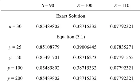
S = 90 S = 100 S = 110
Exact Solution
n = 30 0.85489802 0.38715332 0.07792321 Equation (3.1)
y = 25 0.85108779 0.39006445 0.07835271 y = 50 0.85491701 0.38716273 0.07791555 y = 100 0.85489802 0.38715332 0.07792321 y = 200 0.85489802 0.38715332 0.07792321
in each of the stock price scenarios. For the prices coincide up to the eighth decimal place and there are no noteworthy differences between the two frame- works.
100
y
We conclude the numerical analysis by considering put options in Kou’s double exponential model. The “exact” solution in form of an infinite series can by found in the original article of Kou. The input parameters are the same as above except for the jump component:
1 3.0465, 2 3.0775
and . Table 4
shows the results for the double exponential model.
0.3445
p
Similar to the log-normal model, the numerical appro- ximation of the integral solution produces satisfactory results. The convergence rate is comparable to the pre- vious model.
In summary, the numerical experiments carried out demonstrate that the new framework besides its theoreti- cal insights produces prices with a convincing degree of precision. The Mellin transform approach must be re- garded as a capable alternative to existing methods.
5. Conclusions
The purpose of this paper is to explore the valuation of options where the underlying follows a jump-diffusion. The Mellin integral transform approach was applied to solve the homogeneous PIDE analytically. The proposed solution has a very compact form as one single integral which may be evaluated easily and quickly by quadrature. The final pricing formula offers a powerful and flexible tool for handling a variety of jump size distributions and payoff structures. For log-normally distributed jumps, it was shown explicitly that in case plain vanilla puts our integral expression equivalent to the infinite series solu- tion of BSM-prices.
The numerical results are convincing and logically consistent. They come along with the theoretical findings.
Future research projects are multifaceted. An exten- sion of the proposed approach to American options
Table 4. Prices of European put options in Kou’s model using the infinite series representation with n = 30 and the integral solution from Theorem 3.1.
S = 90 S = 100 S = 110
Exact Solution
n = 30 9.43045738 2.73125890 0.55236304 Equation (3.1)
[image:7.595.57.285.600.736.2]seems to be possible. Also multi-asset options in jump- diffusions could be valued within this framework.
REFERENCES
[1] R. Merton, “Option Pricing When Underlying Stock Re- turns Are Discontinuous,” Journal of Financial Econom- ics, Vol. 3, No. 1-2, 1976, pp. 125-144.
doi:10.1016/0304-405X(76)90022-2
[2] C. Ahn and H. Thompson, “Jump-Diffusion Processes and the Term Structure of Interest Rates,” Journal of Fi- nance, Vol. 43, No. 1, 1988, pp. 155-174.
doi:10.1111/j.1540-6261.1988.tb02595.x
[3] D. Bates, “Jumps and Stochastic Volatility: Exchange Rate Process Implicit in Deutsche Mark Options,” Review of Financial Studies, Vol. 9, No. 1, 1996, pp. 69-107.
doi:10.1093/rfs/9.1.69
[4] D. Madan, P. Carr and E. Chang, “The Variance Gamma Process and Option Pricing,” European Finance Review, Vol. 2, 1998, pp. 79-105.
[5] L. Andersen and J. Andreasen, “Jump-Diffusion Proc- esses: Volatility Smile Fitting and Numerical Methods for Option Pricing,” Review of Derivatives Research, Vol. 4, No. 3, 2000, pp. 231-262. doi:10.1023/A:1011354913068
[6] D. Duffie, J. Pan and K. Singleton, “Transform Analysis and Option Pricing for Affine Jump-Diffusions,” Econo- metrica, Vol. 68, No. 6, 2000, pp. 1343-1376.
doi:10.1111/1468-0262.00164
[7] S. Kou,“A Jump-Diffusion Model for Option Pricing,”
Management Science, Vol. 48, No. 8, 2002, pp. 1086- 1101. doi:10.1287/mnsc.48.8.1086.166
[8] S. Kou and H. Wang, “Option Pricing under a Double Exponential Jump Diffusion Model,” Management Sci- ence, Vo. 50, No. 9, 2004, pp. 1178-1192.
doi:10.1287/mnsc.1030.0163
[9] A. Sepp, “Analytical Pricing of Double-Barrier Options under a Double-Exponential Jump-Diffusion Process: Ap- plications of Laplace Transform,” International Journal of Theoretical and Applied Finance, Vol. 7, No. 2, 2004, pp. 151-175. doi:10.1142/S0219024904002402
[10] K. Amin, “Jump Diffusion Option Valuation in Discrete Time,” Journal of Finance, Vol. 48, No. 5, 1993, pp. 1833-1863. doi:10.1111/j.1540-6261.1993.tb05130.x
[11] J. Hilliard and A. Schwartz, “Pricing European and Ame- rican Derivatives under a Jump-Diffusion Process: A Biv- ariate Tree Approach,” Journal of Financial and Quanti- tative Analysis, Vol. 40, No. 3, 2005, pp. 671-691.
doi:10.1017/S0022109000001915
[12] Y. D’Halluin, P. Forsyth and K. Vetzal, “Robust Numeri- cal Methods for Contingent Claims under Jump Diffu- sion Processes,” IMA Journal of Numerical Analysis, Vol. 25, No. 1, 2005, pp. 87-112. doi:10.1093/imanum/drh011
[13] P. Carr and A. Mayo, “On the Numerical Evaluation of Option Prices in Jump Diffusion Processes,” European Journal of Finance, Vol. 13, No. 4, 2007, pp. 353-372. [14] A. Mayo, “Methods for the Rapid Solution of the Pricing
PIDEs in Exponential and Merton Models,” Journal of Computational and Applied Mathematics, Vol. 222, No. 1, 2008, pp. 128-143. doi:10.1016/j.cam.2007.10.017
[15] S. Clift and P. Forsyth, “Numerican Solution of Two Asset Jump Diffusion Models for Option Valuation,” Ap- plied Numerical Mathematics, Vol. 58, No. 6, 2008, pp. 743-782. doi:10.1016/j.apnum.2007.02.005
[16] R. Panini and R. P. Srivastav, “Option Pricing with Mel- lin Transforms,” Mathematical and Computer Modelling, Vol. 40, No. 1-2, 2004, pp. 43-56.
doi:10.1016/j.mcm.2004.07.008
[17] R. Frontczak, “Valuing Options in Heston’s Stochastic Volatility Model: Another Analytical Approach,” Journal of Applied Mathematics, Vol. 2011, 2011, Article ID: 198469. doi:10.1155/2011/198469
[18] R. Cont and P. Tankov, “Financial Modelling with Jump Processes,” Chapman & Hall/CRC,Boca Raton, 2004. [19] B. Eraker, M. Johannes and N. Polson, “The Impact of
Jumps in Volatility and Returns,” Journal of Finance, Vol. 58, No. 3, 2003, pp. 1269-1300.
![Table 1The parameters were found in [12] and are based on a](https://thumb-us.123doks.com/thumbv2/123dok_us/7825151.732043/6.595.59.289.509.594/table-the-parameters-based.webp)