Tail Dependence Study of SSE Composite Index and SZSE Component Index Based on the Copula

(1)

Tail Dependence Study of SSE Composite Index and SZSE

Component Index Based on the Copula

*

Guohua Sun, Hongliu Su, Guoqiang Tang College of Science, Guilin University of Technology, Guilin, China

Received April 17, 2013; revised May 17, 2013; accepted May 24, 2013

Copyright © 2013 Guohua Sun et al. This is an open access article distributed under the Creative Commons Attribution License, which permits unrestricted use, distribution, and reproduction in any medium, provided the original work is properly cited.

ABSTRACT

With the rapid development of financial industry, copula methods are more and more widely used for the study of financial fields. By selecting the appropriate copulas, the tail dependence of financial variables can be measured easily. Using the nonparametric estimation method to select A12 copula from Archimedean copulas, and do tail dependence study of SSE composite index and SESE component index. The results show that the SSE composite index and SESE component index simultaneously have the upper tail dependence and lower tail dependence, and the upper tail dependence coefficient is less than the lower tail dependence coefficient, which is consistent with the real financial market rule.

Keywords: Rank; Copula; Nonparametric Estimation; Tail Dependence

1. Introduction

With the continuous development of the financial markets, the relationship of interior financial markets is more and more complex, it will promote the study of dependence between financial market structure. In the quantitative analysis of related financial market structure, dependence study is very important, a series of financial problems involve the dependence studies, such as risk management, portfolio selection, asset pricing and so on. Using multivariate distribution function to depict the dependence between each component is the most common method in mathematics; However traditional multivariate distribution function exists some problems in practical application, when the analysis formulas of multivariate distribution function contain many variables, it will be difficult to handle, and it requires the type of marginal distribution function to fit the type of multivariate distribution function. In financial analysis, marginal distribution often do not have the same type of distribution, this makes the traditional multivariate distribution functions can not be widely used in the dependence analysis of financial markets. By Sklar theorem [1], using the copula function to structure flexible multivariate distribution

function, so as to grasp the real dependence between financial markets. Therefore, in this paper we use copula functions to study the tail dependence between SSE composite index and SZSE component index.

At present, using copula function to study the dependence of the financial market already had many achieve- ments, but also in many domestic and foreign literatures, most of them used parameter estimation method to estimate parameters of copula functions. The innovation of this paper is to use a parameter estimation method for parameter estimation, to determine copula functions, and then to do the test of tail dependence.

2. Tail Dependence Based on Copula

Tail dependence can be used to represent extreme events of the interaction between the variables, for example, when the random variable X increased or decreased significantly, the probability of the random variable Y increased or decreased significantly [2]. We use the tail dependence coefficient of copula to research the relationship between SSE composite index and SZSE component index. Let X and Y be continuous random variables with distribution functions F and G respectively, and whose copula is C, and then, based on the copula function we define the upper tail dependence coefficient U and the lower tail dependence coefficient L as follows [3]:

*

(2)

 





 

1

1 lim

1 2 ,

lim 1

U t

t

P Y G t X F t

t C t t

t

 _



 



  

  



(1)

 





 

0

0 lim

, lim

L t

t

P Y G t X F t

C t t

t

 _



 



  

 (2)

where , when , we think the

upper (lower) tail of X_andY be asymptotic dependence; when , we think the upper (lower) tail of X and Y be asymptotic independence; where

 

, 0,

U L

  

 

0

U L

  

1  _U

 

_L 0

 

F t and



G t



 

are the t quantile functions of distribution func- tions F  and G

 

 respectively [4].

3. Selecting Copulas and Estimating

Parameters

There are many kinds of copula functions, Elliptic copulas and Archimedean copulas are used commonly, and each group has many specific copula functions. Different copula functions have different properties, in the actual application, choosing the right copula functions need to follow two principles: one is that the established model of copulas should be easy to operate and understand, to avoid the phenomenon of unknown parameters [5]; sec- ond is to choose the appropriate copula functions which are suitable for the sample datas. Elliptical copula functions are with a symmetrical tail dependence, this will be conflicted with fat-tailed distribution of financial datas. Archimedean copulas are the most widely used in the financial field, and it is easy to build and calculate them. The bivariate normal copula with symmetry and asymptotic tail independence is applied widely, but it is unable to capture the asymmetric dependence and tail dependence between the variables. Here we select copulas which have obvious tail features. Because the log return correlation is accorded with the Archimedean copula distribution, so we choose the Clayton copula with obvious lower tail features, the Gumbel copulas with obvious upper tail features, and the A12 copula with both upper and lower tail features from Archimedean copulas on the financial data fitting [6]. Moreover Archimedean copulas have a feature that Kendall’s tau is the analytic function of . By Sklar theorem, when marginal distribution function is continuous, the copulas function will be uni- quely identified.

For the parameter estimation of a specific copula function, parametric approach and nonparametric approach are common methods: 1) strict maximum likelihood approach (EML) and marginal distribution extrapolation approach (IFM) are more frequently used in the parameter method. Maximum likelihood approach estimates

marginal distribution and parameters of copula function at the same time; Marginal distribution extrapolation approach divide estimation process into two steps, first to estimate the parameters of the marginal distribution function, and then estimate the parameters of copula function. 2) Genest and Rivest approachs are commonly used in the nonparametric approach [7]. As we know, for a copula function C u v

 

, , it is related to the Kendall’s tau as following:

   

 _0,12

4 C u v, dC u v,





1

So for most of the single parameter Archimedean copula functions, because of its generating element 

 

t is a function of the parameter  and the relationship between 

 

t and the Kendall’s tau as follows:

 

1

0 1 4 t dt

t

 



  



(3)

By solving the formula above, we can get the estimate value of . The deficiency of EML and IFM approaches lie in the parameter estimation of copula function is af- fected by the marginal distribution function, if the as- sumptive model of marginal distribution function were wrong, it will lead to a biased estimate to the copula function. Therefore, in this article we use nonparametric estimation method in view of the features of the Archi- medean copulas, to calculate the estimate value of  by the estimate value of the Kendall’s tau, further to estimate the parameters of copula functions.

3.1. The Introduction of Three Types of Copulas

1) Gumbel copula

 



 



1

, exp ln ln , 1

Gu

C u v u v



 

  __    __  (4)

Gumbel copula function is very sensitive to the change of variables at the upper tail of the distribution, so it can quickly capture the changes of upper tail dependence, and it can be used to represent the relations between financial variables which have upper tail dependence. Its parameter  represent the degree of correlation, when

1

 , the variables are independent; when  , the variables are completely related. By formula (1) and (4), we can get the upper tail dependence coefficient of Gumbel copula function, namely _{2 2}1

U



  



t

, by its generating element _

  

t ln  and formula (3), the Kendall’s tau is the analytic function of

  

:

1

 



 

Then, 1

1

 



(3)

1 ˆ ˆ 1   

 (5)

In addition, by the formula

 



 







1 2 ,

1

U P Y G X F

C                 

We can get  U

 

under different levels of . 2) Clayton copula

 





1

, 1

Cl

C_ u v  uv  ,0 (6) Clayton Copula function is very sensitive to the change of variables at the lower tail of the distribution, so it can quickly capture the changes of lower tail dependence, and it can be used to represent the relations between financial variables which have lower tail dependence. Its parameter  also represent the degree of correlation, when  0, the variables are independent; when   , the variables are completely related. By formula (2) and (6), we can get the lower tail dependence coefficient of Clayton copula function, namely ₂ 1

L



 _  , by its generating element and formula (3), the Kendall’s tau is the analytic function of

 

t t  1

  _  _ : 2     

Then, 2

1

 





 , accordingly, ˆ 2 ˆ ˆ 1    

 (7)

In addition, by the formula

 



 





,



L

C

P Y G X F  

   



 

   

We can get  L

 

under different levels of . 3) A12 copula of Archimedean copulas

 



1

 

1



1 1

, 1 1 1 ,

C u v u v

         _ _  _ _    _   

  1



 (8)

Gumbel copula function has only the feature of the upper tail dependence, and Clayton copula function has only the feature of the lower tail dependence, while the A12 copula of Archimedean copulas has both upper tail and lower tail dependence, by formula (1) and (8), the upper tail dependence coefficient can be expressed with

the formula 1

2 2 U



   , and by formula (2) and (8), the lower tail dependence coefficient can be expressed with the formula 1

2 L



 _ 

n by its generating element

 

, the 1 1 t t      

the analytic func

    and formula (3), the Kendall’s tau is

tion of :

2 1 3     Then,



2



3 1



 

 , accordingly,



2



ˆ ˆ 3 1   

 (9)

3.2. Estimating



with Nonparametric Estimation

In order to estimate the parameters, firstly we need to know the estimated value of the Kendall’s tau, originally the Kendall’s tau was not defined by the copula function

 

C  , it was defined by the consistent probability of the random variable



X Y,



minus the non-uniform probability of the random variable



X Y,



, that is



X Y,



P



X1 X



Y2



0



   











2 1

1 2 1 2 0

Y

P X X Y Y



   

where



X Y1, 1



and



X Y2, 2



are independent identi-cally distributed samples of the random variable



X Y,



.

If



X Y1, 1



,,



X Yn, n



are independent identically distributed samples which come from joint distribution function F

 

 of random variable



X Y,



and its copula function is C

  

 , R S1, 1



,,



Rn,Sn



are the ranks of these samples, R ii, 1, 2,,n represent the rank of

, 1, 2, , i

X i n; Si,i1, 2,,n represent the rank of , 1, 2, ,n

i

Y i  as

; then the Kendall’s tau for the sample is defined





1







2



sgn sgn

1 i j n i j i j

R R S S

n n   

  





(10)

So we can work out ˆ

 

ˆ

 on the basis of ˆ, and the copula function can be de rmined solely; then according to the next two formulas to calculate the estimated values of the upper tail dependence coefficient and the lower tail dependence coefficient.

te

ˆ 1 ˆ

U 2 2



   (11) ˆ 1 ˆ ₂ L   _  (12)

4. Computing Steps and Results

4.1. Calculating the Parameter



ˆ

We select day’s closing price



p qi, i



,n1024, of SSE composite index and SZSE component index from Janu- ary 4, 2007 to March 21, 2011. Logarithmic yield



x yi, i







log



pi1 pi



, log



qi1 qi



.





 



We define R Si, i 



rank xi , rank yi



we can get ˆ 0.77338

, and by

(4)

(5 and formula (9) respectively; 3) Putting the which was calculated in step 2) into formula (13);

i t

), formula (7) we get es-

timated values of parameters o ent copulas in Ta- ble 1.

f differ

From Table 1, the parameters of three kinds of copulas are

4) K_C ~U

 

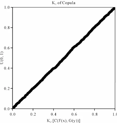
0,1 , to do test with a Q-Q figure of the uniform distribution.

in their respective domains, this explain that there ex

So we use these steps to get the Q-Q test which is shown in Figure 1.

ist both upper tail dependence and lower tail dependence between SSE composite index and SZSE component index. Because the A12 copula of Archimedean copulas has both upper tail and lower tail dependence, we choose A12 copula to study for tail dependence, then we should do the test for the selected copula functions.

4.2. Testing for Copulas

In Figure 1, the K_{C F X G Y}_ _{   }_, _

 

t of A12 copula dis- tribute uniformly on the oblique diagonal line and two sides, so it obey uniform distribution; Table 2 can also explain the K_{C F X G Y}_ _{   }_, _

 

t of A12 copula obeys uniform distribution. Therefore, we think that the A12 copula function is appropriate for describing the relationship between SSE composite index and SZSE component index, namely, A12 copula function is feasible to study the tail dependence of SSE composite index and SZSE component index.

In order to further illustrate A12 copula f scribe the tail dependence be

unction can de- tween SSE composite index and SZSE component index, we do test for the datas. In order to avoid the fault of hypothetical marginal distribution of copula function, we estimate parameters with the Kendall’s tau directly, so we don’t know the marginal distribution function. We use the empirical distribution and KC to structure and test variables which obey uniform distribution on inspection. Firstly we use geometric meth to test copula distribution, then use K-S statistics to do the test of goodness of fit.

4.3. Studying Tail Dependence

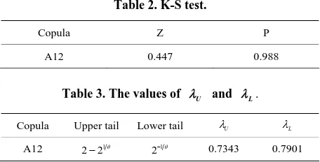
By formula (11) and formula (12), we can work out the upper tail dependence coefficient and the lower tail dependence coefficient, the results are shown in Table 3.

od

Univariate distribution function KC

 

t is defined as

 

_{ }

C

K t  t  t t



where, 

 

t is the generating elem nt of copula func- e tions [8], K_{C F X G Y}_ _{   }_, _

 

t obeys the standard uniform distribution. Setting variables X and Y to obey the empirical distri e can wok out the

   

 

bution, then w

 

,

C F X G Y

K t by means of ˆ. For A12 copula function,

   

 , 

 

C F X G Y

1

1 t

K t t





 _ _

  (13)

 

Follow the steps to calculate,

1) To solve the distribution function F x

 

i and







 

yi of logarithm yield

G



1

i _{ }_{i n} empirical distribution function);

o solve



,

i

x y (b and G

2) T

oth F are



  

,G y



i i i

[image:4.595.310.536.352.590.2]

t C_ F x by formula (8); Figure 1. Q-Q figure of KC function of A12 copula.

Table 1. Parameter estimation of copulas.

 ,

C u v  ˆ ˆ  _ˆ

 



   



1

, exp ln ln

Gu

C u v  __  u  v __ ˆ1 1 ˆ

Gumbel Copula  4.4127

Clayton Copula  





1

, 1

Cl

C u v u v 



 

   _ˆ_₂__ˆ₁___ˆ _6.8253

A12 Copula



 



1 1

1 u 1 v 1



  

 

 __ _ _ _ _ 

 _ _ 

  ˆ2 3 1 ˆ 2.9418

[image:4.595.111.483.636.734.2]

(5)

st.

[image:5.595.58.286.88.204.2]

Copula Z P

Table 2. K-S te

A12 0.447 0.988

able 3. The va

T lues of U and L.

Copula Upper tail Lower tail U L

A12 1

22 1

2 0.7343 0.7901

T able 3 show that the per pen fficient is 0.7343, the lower tail dependence coefficie

he T s up tail de dence co-

e is

nt 0.7901. It indicates that there exists both upper tail dependence and lower tail dependence between SSE composite index and SZSE component index, what’s more, the upper tail dependence is less than the lower tail dependence. The tail dependence between logarithmic yield of SSE composite index and logarithmic yield of SZSE component index demonstrated the consistency of both two extremums; it also demonstrated that whether the price rise or fall, there would be different degrees of dependence between two indices.

5. Conclusion

We select Gumbel copula, ula from Archime

Clayton copula and A12 cop-dean copulas, all of which have fea-tures of tail dependence. We use the nonparametric estimation approach to estimate parameters of copula functions, and find that there exists both upper tail dependence and lower tail dependence between SSE composite index and SZSE component index, therefore, we select A12 copula to do the empirical analysis about the tail dependence between SSE composite index and SZSE component index. The results show that the upper tail dependence coefficient is less than the lower tail dependence coefficient between SSE composite index and SZSE

the downturn of the stock market is higher than the active period, which is consistent with the real financial market rule [9].

com nent index, that is t ay, the dence between SSE posite index and SZSE c ent index during

REFERENCES

[1] R. B. Nelsen, “An Introduction to Copulas,” Springer- Verlag, New Y

po com

o s depen

ompon

ork, 2006, pp. 17-23.

[2] A. Juri and M. V. Wutrich, “Copula Convergence Theo- rems for Tail Events,” Insurance Mathematics and Eco- nomics, Vol. 30, No. 3, 2002, pp. 405-420.

doi:10.1016/S0167-6687(02)00121-X

[3] H. Joe, “Multivariate Models and Dependence Concepts,” Chapman & Hall, London, 1997, pp. 186-198.

doi:10.1201/b13150

[4] A. J. McNeil, R. Frey and P. Embrechts, “Quantitative Risk Management: Concepts, Techniques and Tools,” ceton University Pres

Prin- s, Princeton, 2005, pp. 201-208. [5] J. V. Rosenberg and T. Schuermann, “A General Ap-

proach to Integrated Risk Management with Skewed, Fat- Tailed Risks,” Journal of Financial Economics, Vol. 79, No. 3, 2006, pp. 569-614.

doi:10.1016/j.jfineco.2005.03.001

[6] Y. Li and X. J. Cheng, “Tail Dependence Analysis of SZI & HSI Based on Copula Method,”

Vol. 24, No. 5, 2006, pp. 88-92.

Systems Engineering,

[7] C. Genest and L. P. Rivest, “Statistical Inference Proce- dures for Bivariate Archimedean Copula,” Journal of the American Statistical Association, Vol. 88, No. 423, 1993, pp. 1034-1043. doi:10.1080/01621459.1993.10476372

[8] V. Durrleman, A. Nikeghbali and T. Roncalli, “Which Copula Is the Right One?” Groupe de Recherche Opera- tionelle, Credit Lyonnais, France, 2000, pp. 13-15. [9] X. L. Ren and S. Y. Zhang, “Tail Dependence Analysis of