The impact of medium skilled immigration: a general equilibrium approach

The impact of medium-skilled

immigration: a general equilibrium

approach

Vallizadeh, Ehsan and Joan, Muysken and Thomas, Ziesemer

Maastricht University, Maastricht Research School of Economics of

Technology and Organization (METEOR)

3 July 2012

General Equilibrium Approach

∗

Joan Muysken

Ehsan Vallizadeh

Maastricht University

Thomas Ziesemer

July 11, 2012

Abstract

This paper analyses the impact of the skill composition of migration flows on the host country’s labour market in a specific-factors-two-sector model with heteroge-neous labour (low-, medium-, and high-skilled). We assume price-setting behaviour in both manufacturing and services sectors. The low- and medium-skilled labour markets are characterized by frictions due to wage bargaining. Moreover, we assume bumping down of unemployed medium-skilled workers into low-skilled service jobs whereas endogenous benefits create an interdependency between the two bargaining processes. Particular attention is paid to medium-skilled migration which enables us to augment the literature by replicating important stylized facts regarding medium skills, such as i) the interaction between immigration, low-skilled unemployment and medium-skilled over-qualification, ii) the polarization effect where both low-and high-skilled wages increase relative to the medium-skilled. The model is cali-brated using German data. The key findings are: (i) a perfectly balanced migration has a neutral impact on the receiving economy due to international capital flows; (ii) immigration of medium-skilled labour together with some high-skilled labour low-ers the low-skilled unemployment rate and has a positive effect on output per capita; (iii) migration of only medium-skilled labour has a neutral GDP per capita effect.

Keywords Medium-Skilled Migration·Wage and Price Setting·Specific Factors Model·Unemployment·Over-qualification·Wage Polarization

JEL F22·J51·J52·J61·J64

∗_{We thank for helpful comments of participants at NAKE Research Day 2011 at the University of}

Utrecht as well as at the 17th Spring Meeting of Young Economists at the ZEW in Mannheim 2012. †_{j.muysken@maastrichtuniversity.nl}

1.

Introduction

The admission of ten Central and Eastern European countries (CEECs) into the

Euro-pean Union has made the incumbent member states worried about the adverse economic

consequences due to potential mass migration from those countries.1 This has lead to

transitional restrictions − with UK, Sweden, and Ireland as exceptions − on the free

movement of workers vis--vis new member states. With the end of the transitional

pe-riods as of May 2011 the debate concerning the East-West mass migration has revived

in countries like Germany and Austria, the closest countries to those new members, that

had fully prolonged the transitional periods up to seven years. The main rationale for this

restrictive action and the general concerns is explained by the perception regarding the

adverse consequences for the natives, particularly, for the least skilled workers (cf. for a

surveyDustmann et al.(2008)).2 The empirical evidence on the labour market impact of

migration is rather mixed and clusters usually around zero.3 However, widely recognized

phenomena in the literature on the economic impact of immigration are that high-skilled

immigrants have a positive influence on GDP growth and employment, while low-skilled

migrants have a negative influence.4

Economic theory provides clear grounds for both phenomena, although the

appropri-ateness of the empirical approach has been questioned and criticized (seeBorjas(2003)).

The displacement effect of native workers due to immigration can be explained by two

main forces: i) the substitution effect, and ii) the “crowding-out” effect. While the former

denotes the shifts in the relative factor demand determined by the underlying

produc-tion technology, the second effect emphasizes the shifts in the labour supply that might

displace the least skilled from the labour market. This paper incorporates both effects.

The empirical evidence indicates, in fact, that immigrants face a higher risk of

over-qualification, i.e. they perform jobs for which skill requirement is less than their

qualifi-1_{On 1 May 2004, eight CEECs, the Czech Republic, Estonia, Hungary, Latvia, Lithuania, Poland,} Slovakia, and Slovenia plus two Mediterranean countries Malta and Cyprus joined the EU with Bulgaria and Romania followed on 1 January 2007.

2_{See alsoBoeri and Brcker(2005) who emphasize the concerns regarding welfare-effects.}

3_{The empirical studies looking at the post-accession effects for the UK labour market could not find any} significant impact on native wages and unemployment (cf. Gilpin et al.(2006),Lemos and Portes(2008),

cation−seeOECD(2007) for a cross-country evidence andDrinkwater et al.(2009) for

UK.

Surprisingly enough, very little attention is paid to the impact of medium-skilled

mi-grants as a separate category, although nowadays they constitute the major component of

immigrants and employees.5 This paper seeks to correct this omission by analysing the

impact of immigration in a two-sector model, with three types of skills. We assume

wage-and-price-setting behaviour in both manufacturing and services sectors. This enables us

to augment the literature by replicating important stylized facts regarding medium skills,

such as i) the interaction between immigration, low-skilled unemployment and

medium-skilled over-qualification, ii) the so called polarization effect where both low- and

high-skilled wages have increased relative to the medium-high-skilled wages.6

A seminal way of analyzing the impact of immigration on output, wages and (un)employment

has been introduced by Borjas(2003) andOttaviano and Peri(2008, 2011) for the U.S.

economy. They use a production function in which output is produced utilizing capital

and labour, while labour is defined by a multi-level-nested (skill-experience-nationality)

CES composite − a common approach in the labour markets studies (cf. Card and

Lemieux(2001)). From this function demand for labour is derived, and the market

clear-ing wage results from equality with exogenous labour supply. Since in the European

context labour markets usually do not clear, in particular not when immigration is

in-volved, several recent papers analyse the wage and (un)employment effects of migration

for imperfect labour markets. Three recent papers in this field areBrcker and Jahn(2011),

D’Amuri et al.(2010), andFelbermayr et al. (2010), which all apply to the case of

Ger-many. All three studies use the multi-level nested CES production function to derive

demand for labour. However, instead of competitive wages, they introduce a wage setting

curve where wages for a certain skill are negatively related to unemployment in that skill

group. Using data for Germany, they estimate the elasticity of substitution between the

different education-experience groups as well as between natives and foreigners.

More-over, they estimate the unemployment elasticity of wages. Given these estimation results

they then simulate the impact of immigration on wages and (un)employment of each sub

5_{Since we match our model with German data using theEU KLEMSdata set, the different skill groups} are defined as follows. High-skilled: University graduates, Medium-skilled: Intermediate qualifications, and low-skilled: No formal qualifications, seeTimmer et al.(2007).

group.7

All these studies, however, focus mainly on two types of migration scenarios in the

simulation of their models: low-skilled or high-skilled migration flows. The overall

re-sult from these studies is that incumbent immigrants are mostly hurt by new immigrants,

while natives are positively (or at least neutrally) affected in the long-run. We hope,

there-fore, to provide new insights by adding interesting labour market features such as wage

determination through multiple sectoral bargaining processes interconnected by bumping

down and endogenous benefits.

We, therefore, pursue a different route, which essentially opens the black box of a

multi-level-nested CES to describe the substitution possibilities. In our approach, we

specify a specific-factors two-sector model, with three types of labour. Motivated by our

stylized facts which will be presented below, the manufacturing sector employs medium

and high-skilled labour, while the service sector employs low and high-skilled labour

in both cases next to capital. This model resembles to some extent that of Felbermayr

and Kohler(2006,2007) who examine the immigration effect for heterogeneous and

per-fectly competitive labour markets (low, medium, and high skill levels) and allow for

inter-industry trade in a similar specific-factors model. However, in our model we allow for

both wage bargaining and price setting in both sectors, which allows for unemployment

of low skilled workers and bumping down of medium skilled workers to low skilled jobs.

The advantage of this approach in our view is that the substitution between types of

work-ers is less mechanical when compared to the multi-level CES, and less rigid over time.

We allow for economic mechanisms to play a role due to shifts in the sectoral

composi-tion of the economy and substitucomposi-tion between labour and capital within sectors, next to

bumping down of medium skilled workers to low skilled jobs. Moreover, this approach

allows us to focus on the impact of medium skilled immigration, which is the dominant

type of immigration nowadays (see Table1), but largely ignored in the literature. The fo-cus on medium skilled migration is important not only from an economic point of view,

but also from a policy perspective. High-skilled immigration is not controversial due to

its commonly accepted and well documented beneficial impact on the receiving country.

Politically less accepted are policies in favour of unskilled immigration, simply because

7_{As shown recently byOttaviano and Peri(2011), the elasticity of substitutions between different} skill-age groups is significantly affected by the nesting structure of the labour composite. See alsoBorjas et al.

of its perceived adverse welfare and economic effects. Therefore, as we show below, the

neutral impact of medium-skilled labour migration induces an interesting policy

implica-tion for the future labour shortage problems indicating the permanent outflow from the

labour market, e.g. due to ageing.

The set up of the paper is as follows. The next section presents the stylized facts on

migration pattern, labour market composition, and trends in employment and wages in

the manufacturing and service sectors for Germany. In section 3. we demonstrate the theoretical framework with two major sectors, three skill groups and a double wage

bar-gaining model determining the wages of medium- and low-skilled labour. In section4., we provide first a qualitative assessment of the comparative static analysis, derived by

means of log-linearisation around the steady-state, followed by an intuitive interpretation

of the theoretical results. In section5., we calibrate the model for Germany using the EU-KLEMS data set to measure the quantitative importance of various migration scenarios.

Finally, section6. presents the concluding remarks.

2.

Stylized facts

At the aggregated level, the average impact of immigration on unemployment and wages

of native workers has been explored quite extensively and tend to cluster around zero,

as discussed above. However, as already emphasized, the literature on migration has

somehow ignored the potential impact of medium-skilled work force, although it accounts

for a large part of the total labour force as well as of the foreign work force nowadays.

Table1highlights this feature in the case of Germany by showing the composition of the total labour force across manufacturing and service sectors as well as of the foreign labour

force by skill groups for the years 1991 and 2005. Noticeable, the most pronounced

increase was in the share of foreign medium-skilled labour.

Another phenomenon that has recently attracted the attention is the job polarization

phenomenon in many developed countries. Table 2 presents this for Germany where we show the percentage changes in the total employment shares as well as in the wage

rates by education and industry for the period 1991-2005. One sees clearly that

high-skilled employment shares increased in both sectors, whereas the low-high-skilled share in

low-Table 1: Total and foreign labour force, by education groups

1991 2005

Total Mig. Total Mig.

Skills Agg. Manuf. Serv. Agg. Manuf. Serv.

High (%) 8 6 9 4 10 7 10 6

Medium (%) 64 63 65 48 62 66 61 61

Low (%) 28 31 25 48 28 27 28 33

Notes: Agg.=Aggregate, Manuf.=Manufacturing, Serv.=Services, Mig.=Migrants. The total shares denote the shares in hours worked, and are calculated from EU KLEMS. The number for foreigners are taken fromBrcker and Jahn(2011), but denoting, respectively, the years 1990 and 2004. Medium-skilled consists of the educational groups: vocational and high-school.

and high-skilled wages grew faster relative to medium-skilled wages reflecting the

U-shaped trend found in the empirical literature (see, for example,Autor and Dorn(2010)

for the U.S. and Goos et al. (2009) for Europe). While the main rationale behind this

trend is explained by the advances in information and communication technology (see,

for instance,Van Reenen et al.(2010)), this paper gives an alternative explanation. We

show that it might also be due to relative increase in the medium-skilled labour force due

to migration. This brings us to the next stylized fact.

A study by OECD (2007) documents that the labour market performance of

im-migrants is denoted by higher risk of over-qualification. Recent studies on

post-EU-enlargement provide further evidence. For example, Drinkwater et al. (2009) analyse

the performance of Polish immigrants in the UK labour market and find that majority of

them are employed in low-skilled and low-paid jobs despite having relatively high levels

of education.8

Moreover, a recent study by Brynin and Longhi (2009) finds for Germany, using

households survey data, a relative excess of over-qualification at the medium-skilled level

which contributes to almost half of all overqualified persons. This indicates that beside

the standard argumentation of denoting the technical change as the main deriving force

Table 2: Changes in wage rates and employment shares, by education and industry

1991−2005

Wage Rate Employment Share

Manufacturing Sector (in%)

High 59 25

Medium 40 4

Low 42 −15

Service Sector (in%)

High 44 13

Medium 36 −7

Low 41 5

Notes: The numbers denote log-differences. Employment shares designate the shares in hours worked.Source: EU KLEMS.

behind the increase in low-skilled unemployment rate, the increase in the low-skilled

unemployment rate might be the consequence of an increase in supply of better educated

workers leading to the so called “crowding-out” of low-skilled workers. Using German

data, Figure1 shows the relation between low-skilled unemployment rate and the over-qualification rate of low-skilled type of jobs. Except for 2000-2004 (the ICT bust period)

where a positive relation can be seen, it designates a reverse relation, especially, in the

recent years. This observation might be the result of the 2005 labour market reforms in

Germany, the so-calledHartzreforms.

We summarize these stylized facts as follows

1. Medium-skilled workers constitute a major component of the labour force and of

immigrants

2. High-skilled employment rises in both sectors with low-skilled declining in

man-ufacturing sector and medium-skilled in service sector

3. Medium-skilled labour has a higher incidence of over-qualification

4. There is a negative relation between the over-qualification rate in low-skilled jobs

Figure 1: Trends in low-skilled unemployment and over-qualification rates

Note: The over-qualification (OQ) rate denotes the proportion of medium-skilled workers in low-skilled jobs.Source: Eurostat.

5. Both low-skilled and high-skilled wages have increased relative to the

medium-skilled wage, which points at wage polarization

3.

The theoretical framework

The economy is defined by two major sectors,manufacturing(Ym) andservices(Ys), each

producing a good by utilizing physical capital and labour. These two goods are in turn

used in a CES aggregate to produce a final consumption good (X). We interpret X as

the total GDP which is taken as the numeraire, i.e. its price is set to unity. The CES

aggregate can be interpreted as the production technology of a final good sector or as the

utility function of a representative household. In light of the stylized facts reported in

skilled labour to low skilled service jobs can occur. Capital and high-skilled labour are

employed in both sectors. We assume that firms in manufacturing and services sectors

have a monopoly power which is ensured by a fixed entry cost. The high skilled wage

is determined on a competitive labour market, but medium and low skilled wages are

determined by wage bargaining. We elaborate these points below in the context of a

general equilibrium framework.

3.1.

Final consumption good

The final consumption good (or the GDP) is produced by the following CES function

X =

γY

θ−1

θ

m + (1−γ)Y θ−1

θ s

_θθ₋₁

(1)

whereθ >1 denotes the elasticity of substitution between the two sectors and 0<γ <1

is the distribution parameter.

From (1), we obtain the isoelastic demand functions for manufacturing and service goods

Y_md=γθX

Pm

P −θ

(2a)

Y_sd= (1−γ)θX

Ps

P −θ

(2b)

respectively, whereP= (1−γ)θP_s1−θ+γθP_m1−θ 1

1−θ _{denotes the macroeconomic price}

index which is taken as numeraire in the remaining part of the analysis. As a consequence

all variables are defined in real terms and we assume no inflation.

3.2.

Manufacturing and services goods

After incurring a fixed cost, firms in both sectors produce a good with a standard

Cobb-Douglas production technology with constant returns to scale. Note that positive profits

are ensured simply by the assumption of relatively high fixed costs such that free-entry

is ruled out, see Cahuc and Zylberberg (2004, Ch. 7) for a general discussion. Based

labour are employed, whereas in the service sector high- (Hs) and low-skilled (L) labour

are utilized.

The production functions for manufacturing and services are given by

Ym=AKmνHmαM1−α−ν (3a)

Ys=BKsηH

β

s L1−β−η (3b)

respectively, where 0<{α,β,ν,η}<1. The total factor productivity in

manufactur-ing and services is denoted by exogenous variables A and B, respectively, with A>B

reflecting the higher productivity of manufacturing relative to services.

3.3.

Factor demand

Firms determine factor demand by minimizing their costs given the factor prices. The

rental cost of capital, r∗, is determined on the international capital market since capital

is assumed to be perfectly mobile. Furthermore, high skilled workers are assumed to be

mobile between the service and manufacturing sectors. As a consequence the high-skilled

wage is equalized between the two sectors: wm_H=ws_H =wH. The wage bargaining in the

medium skilled and the low skilled labour markets determine wM and wL, respectively.

Factor demand, then, is determined by minimizing the manufacturing production costs

Cm=wHHm+wMM+r∗Km (4)

subject to production technology (3a). Similarly, factor demand in the service sector is determined by minimizing the service production costs

subject to the production technology (3b). Solving the optimization problems, the factor demand functions in the manufacturing sector are given by

H_md =αYm

A w_H

Wm

−1

(6a)

Md= (1−α−ν)Ym A

w_M Wm

−1

(6b)

K_md =νYm

A r∗ Wm −1 (6c)

and in the services sector by

H_sd=βYs

B w_H

Ws

−1

(7a)

Ld= (1−β−η)Ys B

w_L Ws

−1

(7b)

K_sd=ηYs

B r∗ Ws −1 (7c)

whereWm=r_ν∗ν wH

α

α wM 1−α−ν

1−α−ν

andWs=r_η∗ηwH

β

β

wL 1−β−η

1−β−η

de-note the geometric weighted average factor price composite in the manufacturing and

services sectors, respectively.

Substituting (6a)-(6c) into the cost function, (4), and similarly (7a)-(7c) into (5), we obtain the minimized cost functions

C_m∗(wH,wM,r∗) =

Wm

A Ym (8a)

C∗_s(wH,wL,r∗) =

Ws

B Ys (8b)

for manufacturing and service good producers, respectively.

3.4.

Price setting for intermediate goods

As shown in the previous section, firms in the two major sectors face a downward-sloping

domestic demand function for their products. Therefore, a representative manufacturing

good producer sets the price of her good by maximizing her profit

subject to (2a). Similarly, a representative service good producer maximizes her profit

Πs=PsYs−Cs∗(Ws,Ys) (10)

subject to (2b). Solving the maximization problems, yield the standard pricing behaviour, respectively, in the manufacturing and service sectors

Pm= θ θ−1

Wm

A (11a)

Ps= θ θ−1

Ws

B . (11b)

3.5.

Wage setting and the labour market features

As discussed above, high skilled workers are mobile between the two intermediate

sec-tors, and we assume labour market clearing for them. However, in line with the

Euro-pean labour market institutions, wage bargaining occurs in both low- and medium-skilled

labour markets - see, for example,Brcker and Jahn(2011) where wage-setting curves

dif-fer across sectors. In our framework two difdif-ferent labour unions negotiate the wages for

medium- and low-skilled workers in the manufacturing and services sectors, respectively.

But, as we elaborate below, wages are not independent. On the one hand medium skilled

workers can be bumped down into the service jobs, earning low-skilled wages, which

influences the reference wage of medium skilled workers. On the other hand, medium

skilled wages will have an impact on the level of the benefits, which will influence the

reference wage of low skilled workers.

FollowingBooth(1995) andLayard et al.(2005), wages are determined by the

right-to-managebargaining solution so that the negotiating parties only bargain over the wages,

whereas the optimal employment decisions is made by the firms. In doing so, we also

follow the conventional way by assuming that in each sector there exists a continuum of

identical firms and unions and therefore neglect firm-union-specific indices (cf.Koskela

and Stenbacka,2009, 2010). Firm’s net gain is simply the flow of profits, i.e. net of the

fixed costs. This is given for the manufacturing and services firms, respectively, by the

and service labour unions is given, respectively, by

Um = (wM−w¯M)M (12)

Us = (wL−w¯L)L (13)

where ¯wj,∀j=L,M denotes the outside option which is taken as given by each labour

union. Thus, the medium-skilled wage is the result of the following maximization

prob-lem

max

wM ΩM

= (wM−w¯M)Md

δm

Π1−δm

m s.t.(2a),(6b),(9),(11a)

Similarly, the low-skilled wage is set by solving the following maximization problem

max

wL ΩL

= (wL−w¯L)Ld

δs

Π1−δs

s s.t.(2b),(7b),(10),(11b)

whereδi (i=s,m) denotes the bargaining strength of the labour union. The solution of

the wage negotiation yields, after some manipulation, the standard result

wj = (1+λi)w¯j ∀ j=M,L (14)

where the mark-up on the medium- and low-skilled outside options is given, respectively,

by

λm= δm

(1−α−ν)(θ−1) (15a)

λs= δs

(1−β−η)(θ−1). (15b)

3.5.1. Manufacturing wage curve

As shown by the stylized facts, medium skilled workers have a relatively high incidence

of over qualification. Several empirical studies suggest that a significant and increasing

proportion of low-skilled jobs are nowadays carried out by better educated, over-qualified

workers - seeBorghans and de Grip(2000) andHartog(2000) for an overview of these

studies.

risk of holding a low-skilled job in the services sector when they cannot find employment

in the manufacturing sector. As a consequence, they will lead the low-skilled workers

into unemployment. This suggests that the rise in low-skilled unemployment would not

only be the result of a relative demand shift, but also the consequence of a relative supply

shift which leads to “crowding-out” of low-skilled workers as has also been observed by

Pierrard and Snessens(2003).

The medium-skilled over-qualification rate is defined by

oM = 1−

M NM

(16)

withNM as the total medium-skilled labour force.

Since frictions in the medium-skilled labour market is described by the over-qualification

risk, then in the general equilibrium context as well as by the symmetry assumption, the

reference wage of a medium-skilled worker ( ¯wM) can be interpreted as:

¯

wM = (1−oM)wM+oMwL. (17)

Substituting this expression into (14) and rearranging, we obtain the manufacturing wage curve (WCm)

wM=Φ(λm,oM)wL, (18)

where_Φ(λm,oM) =₁₋₍(₁1₊+_λλ_mm₎₍)o₁M_−oM). That is, as long as the manufacturing union has some

bargaining power,δm>0, it will set a markup denoted by_Φ(·)over the low-skilled wage

rate. If, however,δm→0, thenλm→0 andwM →wL denoting the perfect competition

case. One can easily show that ∂Φ/∂oM <0 implying the wage curve is increasing in

3.5.2. Service wage curve

The low-skilled unemployment rate is defined by:9

uL = 1−

L−oMNM

NL

(19)

withNL denoting the total low-skilled labour force.

Contrary to manufacturing, low-skilled workers face the risk of being unemployed

and thus receiving an unemployment benefit,b. Recalling the symmetry assumption, the

outside option (or the average income) of the low-skilled workers is defined as:

¯

wL= (1−uL)wL+uLb (20)

Furthermore, we assume that the level of benefits is tied closely to the average wage which

is in line with the evidence. Weiss and Garloff(2009), for example, show that the level

of benefits is tied closely to per-capita income in most European countries while in the

Anglo-Saxon countries there was no adjustment over the last two decades. Consequently,

we definebas a percentage (ξ) of average low- and medium-skilled wages weighted by

κ:10

b=ξ(κwM+ (1−κ)wL). (21)

Using this definition forbin (20) and substituting then the resulting equation in (14), after rearranging, we obtain the following aggregated service wage curve (WCs)

wL = Ψ(λs,uL)wM (22)

where_Ψ(λs,uL) =_(1+λ (1+λs)ξ κuL

s)(1−ξ(1−κ))uL−λs. Similarly to the manufacturing wage curve, one

can verify that∂Ψ/∂uL<0. Hence the wage curve is increasing in the employment of

9_{Note, the service trade union does not take into account the crowding-out effect when negotiating over} the wage rate and therefore, theperceivedunemployment rate is simply given byu_Lp=1− L

NL.We use this

property in the analysis of the interaction between the service and manufacturing wages.

low-skilled workers. Note that if the service labour union looses the bargaining power,

then the perfect competition outcome with no unemployment results, i.e. ifδs→0, then

λs→0 andwL→b.

3.6.

Interaction between low- and medium-skill wages

Due to the risk of over-qualification and the endogenous unemployment benefits, there is

an interdependency between the low- and medium-skill wages. We show that the

condi-tion for the unique equilibrium is assured by the fact that both wage curves are

monoton-ically increasing in the wage rates, starting from positive intercepts. However, the latter

requires lower boundaries on both unemployment and over-qualification rates. Moreover,

both curves should intersect such that the following relation is ensured,wM >wL>0 .

We now elaborate on the shape and properties of both wage curves derived in the

previous section.

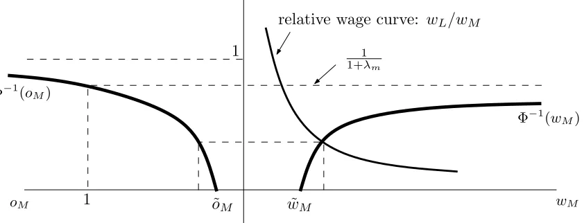
3.6.1. Properties of manufacturing wage curve

The partial features of the manufacturing wage curve (i.e. taking wL as given), can be

demonstrated as follows. For a better realization, rewrite (18) as

wL

wM

=_Φ(λm,oM)−1≡1−

¯

λm

oM(wM)

(23)

where ¯λm= λm

1+λm and oM(wM) is given by (16). Now, the LHS and RHS can both be

seen as a function ofwM for given values ofwL. This is because manufacturing unions

take the outside option (wL) as given when they negotiate. Then, it can be easily verified

that the LHS of (23) is a decreasing function ofwM but the RHS is increasing for certain

values of bothoM andwM, as will be discussed below. These relationships are illustrated

in Figure2.

Consider first the right panel of Figure 2. Then, recalling (18), we can draw two curves: one shows the negative relation between the relative wage rate due to changes

in wM (LHS of (23)) holding the low-skilled wage fixed; the second curve illustrates

the positive relation between the inverse-wage-mark-up function (_Φ−1) and the

medium-skilled wage rate (wM). This relation follows from the positive relationship between

Figure 2: Properties of manufacturing wage curve

w_M 1

1 1

1+λm

relative wage curve: wL/wM

o_M

Φ−1_(w

M)

Φ−1_(o

M)

˜

oM w˜M

decline in the labour demand and increase, thus, the risk of over-qualification. Recalling

the medium-skilled labour demand (6b) and the over-qualification rate (16), then, one can verify the limit cases

lim

wM→∞

Md=0 ⇒ lim

wM→∞

oM=1 ⇒ lim

wM→∞Φ

−1₌ 1

1+λm

.

The intersection between the two curves in the right plane will determine the equilibrium

over-qualification rate and medium-skilled wage level for changes in the low-skilled wage

rate. We conclude

Lemma 1. Positive wages are ensured iff oM ∈(o˜M,1).

Proof. The proof is rather straight forward. Due to the non-negativity assumption of the

wage rates, it follows from (23):

Φ−1 > 0 ¯

λm

oM

< 1

oM > o˜M≡ λm

1+λm

wM > w˜M≡

(1−α−ν)(r/ν)ν(wH/α)α

NM

(1+λm)Ym

A

_α+1_ν

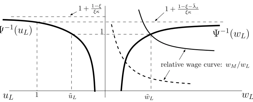
3.6.2. Properties of service wage curve

Similarly, the partial behaviour of the service wage-curve can be assessed as follows.

First, rewrite (22) as

wM

wL

=Ψ(λs,uL)−1≡1+

1−ξ ξ κ −

¯

λs ξ κuL

(24)

where ¯λs= λs

1+λs. With the same intention described above, we define both the LHS and

RHS of (24) as functions of wL for given values ofwM. The argumentation is analogue

to one on the manufacturing wage curve. Thus, we can define two curves with opposite

relations to changes in wM as shown in the right plane of Figure (3), whereas the left

plane shows the relation between (_Ψ−1) and the unemployment rate (uL).

Figure 3: Properties of service wage curve

w

1 + 1−ξ

ξκ 1 +

1₋ξ−λ¯s

ξκ

relative wage curve: wM/wL

u

Ψ

(

w

)

Ψ

(

u

)

˜

uL w˜L

However, the condition that must be satisfied in this case is summarized by the

fol-lowing lemma.

Proof. From (24), it follows:

Ψ−1 > 1 ¯

λs

uL

< 1−ξ

uL > u˜L ≡

¯

λs

1−ξ

wL > w˜L ≡

"

(1−β−η)(r/η)η(wH/β)β

((1−q)NL)

Ys

B #_β+1_η

whereq≡(1− λ¯s

1−ξ). For the last inequality we used the definition of perceived

unem-ployment rate (explained in footnote 9), and the low-skilled labour demand (7b). This implies that for values of unemployment rateuL∈(0,u˜L]the relation between low- and

medium-skilled wage rates is violated, i.e. wM ≤wL. Therefore, to ensurewM>wL, the

unemployment rate must be strictly larger than the lower boundary ˜uL.

Now, from these conditions, the unique intersection of the two wage-setting curves

can be shown graphically in the (wM,wL)-plane. By Lemma 1 and 2, wM > wL >0.

This indicates that in the (wM,wL)-space the wage relation should always be above the 45

degree line. Starting withWCm, one sees from the RHS plane of Figure 2that for large

values of the low-skilled wage rate, the medium-skilled equilibrium wage rises along the

Φ−1 curve due to upward shifts of the relative wage curve. Hence, higherwL increases

equilibrium wM and with it the over-qualification rate which converges to 1+λm, the

reciprocal of the limit shown in Figure2.

Analogously, the derivation ofWCs can be explained by recalling the RHS of Figure

3. Now, changes in wM are associated with moving along the Ψ−1 curve. However,

as explained above, the necessary condition requires that _Ψ−1 >1 for wL >w˜L. This

indicates that in (wM,wL)-space theWCsmust start above the 45 degree line. As described

above, higher wM leads to higher wL along the Ψ−1 curve converging to the limit 1+

1−ξ−λ¯s

ξ κ . However, it should be noted that in the (wM,wL)-plane, the inverse service wage

curve is drawn. To ensure a unique equilibrium, 1+1−ξ−λ¯s

ξ κ >1+λmmust hold which

Figure 4: Unique equilibrium

W Cs

W Cm

1 +λm

1 +

ξκ

w

w

M

w

w

45

˜

w

˜

w

Lemma 3. A unique intersection between the two wage curves is ensured for all

ξ <ξ˜≡ 1

1+λs

1 1+κλm

.

In Table3, we summarize these conditions and assume that they hold.11

An illustration of the interdependence process is that an increase in productivity of

manufacturing, relative to that of services, increases the wage rate in the services sector

without any justification by the corresponding productivity increases in the latter. This

phenomenon is also widely recognized as the main cause of the so-calledBaumol’s

dis-ease, which refers to the increasing share of services relative to manufacturing in an

advanced economy - see, for instance, Hartwig (2011). It also corresponds to the

ob-servation that the low wage differentiation in the Continental Europe is attributed to the

centralization and coordination of wage formation (Siebert,1997).

Table 3: Equilibrium Conditions

Parameter/Variable Range Condition

oM ∈(o˜M,1)

Lemma1

wM >w˜M

uL ∈(u˜L,1)

Lemma2

wL >w˜L

ξ <ξ˜ Lemma3

4.

The General Equilibrium Solution

In this section we present the general equilibrium comparative static analysis. The

ap-proach we choose is the following: First, we derive the changes from the initial

equilib-rium. We then give the intuitive interpretation of the results followed by a summary of

the general equilibrium repercussions on the over-qualification and unemployment rates

as well as on the relative wages.

4.1.

A theoretical assessment without capital input

Following the standard approach pursued byJones(1965), the comparative static analysis

can be assessed by means of log-linearization to denote changes from the initial

equilib-rium, i.e. ˆx=ln x+_xdx

≃dx/x.

By the Le ChatelierSamuelsonprinciple, ignoring capital will only affect the results

quantitatively, but not in qualitative terms, see Felbermayr and Kohler(2007). For that

reason, and for convenience, we simplify the analysis by setting ν =η =0, and thus

reducing the model to a two-factor production function with labour as the only input

factor.

To begin with, take the total differentiation of the log-difference of the labour demand

functions (6a) and (6b), (7a) and (7b), to obtain

ˆ

ˆ

wH−wˆL=Lˆ−Hˆs (25.2)

Linearising the equilibrium conditions for the low- and medium-skilled labour markets,

L= (1−uL)NL+oMNM andM= (1−oM)NM, as well as the market clearing condition

for the high-skilled labour, yield

ˆ

L=l(_Nˆ_{L−u¯LuˆL) + (1−l)(N}ˆ_{M+oˆM) (25.3)}

ˆ

M= (NˆM−o¯MoˆM) (25.4)

ˆ

NH=hHˆm+ (1−h)Hˆs (25.5)

where ¯uL =₁₋uL_uL, ¯oM= ₁₋oM_oM, andh= H_NHm. Note that changes in the low-skilled

employ-ment are weighted byl= (1−uL)NL

L . Similarly, log-linearisation of the wage curves (18)

and (22), yield

ˆ

wM−wˆL=εmoˆM (25.6)

ˆ

wL−wˆM=εsuˆL (25.7)

whereεm=−λ¯m

oMΦ(·)andεs =− ¯

λs

ξ κuLΨ(·)denote the wage curve elasticities. From the

price-setting definitions (11a) and (11b) we obtain

ˆ

Pm= (αwˆH+ (1−α)wˆM) (25.8)

ˆ

Ps= (βwˆH+ (1−β)wˆL) (25.9)

Log-linearisation of the intermediate goods demand equations, (2a) and (2b), yields

ˆ

Ym=Xˆ−θPˆm (25.10)

ˆ

Ys=Xˆ−θPˆs (25.11)

Changes in the total output can, then, be determined by log-linearising (1) which yields

ˆ

X =ϕxYˆm+ (1−ϕx)Yˆs (25.12)

with ϕx =γ Ym

X

σx

= PmYm

production functions (3a) and (3b), respectively, yields

ˆ

Ym=αHˆm+ (1−α)Mˆ (25.13)

ˆ

Ys=βHˆs+ (1−β)Lˆ (25.14)

This system of fourteen equations, (25.1)-(25.14), allows for the assessment of the general equilibrium effects on the fourteen endogenous variables ˆX,_Yˆ_m,Yˆ_s,Pˆ_m,Pˆ_s,Hˆ_m,Hˆ_s,Mˆ_,Lˆ_,oˆM,

ˆ

uL,wˆH,wˆM,wˆL.

4.2.

Comparative static analysis

In this section we examine the impact of an exogenous increase in the labour supply,

which we attribute to immigration in each of the labour markets of our model.

Particu-larly, we are interested in the repercussions on the low- and medium-skilled labour

mar-kets and on output. Intuitively, the wage-setting mechanism reveals that any exogenous

increase in the labour endowments worsening (or improving) the labour market

condi-tion for one of the unionised labour,ceteris paribus, has also consequences for the other

unionised labour. This is due to the fact that an increase inoM(oruL) will force the unions

for wag restraint. Therefore, the wage indexation between both medium- and low-skilled

unionised workers, resulting from the double bargaining mechanism as well as the

en-dogenous unemployment benefits, implies that the outside option of the other unionised

labour market will be affected too. Note that the bumping down effect has an additional

direct impact on the low-skilled wages asuLincreases, see Eq. (19).

Accounting for the general equilibrium repercussions, however, we find that the wage

restraint behaviour induces a higher labour demand for that type of labour. This is

accom-panied by changes in the allocation of high-skilled labour across the sectors as well as in

the demand for goods due to goods price effects. As we show below, the crucial factor

that determines the qualitative impact of migration reveals to be the factor cost share of

the high-skilled labour. In what follows, we omit the formal proofs and provide instead

the economic intuition of the results.12.

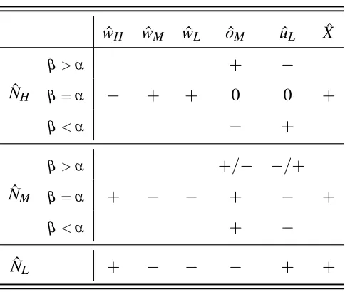
The first interesting outcome of the analysis regarding changes in the wages as well

as in unemployment and over-qualification rates is the following

Proposition 4. A proportional increase in supply of all three skill groups is consistent

with no change in the wages as well as in over-qualification and unemployment rates.

The proportional increase of the labour force implies a scale effect as more resources

are available in the economy to utilize. Note, however, that the marginal productivity of

labour, the high-skilled labour reallocation, the output expansion of both sectors all

de-pend on the size of(α−β), as we show below when discussing migration of each type

of labour separately. Intuitively, for similar cost shares of the high-skilled labour across

the two sectors, i.e. (α−β)→ 0, both sectors expand symmetrically due to

propor-tional changes in the production costs, or alternatively in the marginal productivity, and

thus inducing constant relative goods prices. Therefore, X, Ym,Ys, L andM all increase

approximately proportionally. As shown in the last column of Table4, the impact of mi-gration of any skill group onX is always positive. Thus, setting ˆX =0 does not affect the

results qualitatively, and allows for a better exposition of the driving forces behind the

immigration effects.

Next, we discuss the qualitative effects of an exogenous shock of each of the skill

groups separately on low- and medium-skilled labour markets. An alternative way to

demonstrate the effects on the unemployment and over-qualification rates is to reduce the

system of equations derived in the previous section and to solve it for ˆoMand ˆuL. In doing

so, we obtain the following expressions13

ˆ

oM =

(θ−1)θ

ζ (β−α)wˆH−

(β+θ(1−β))−(α+θ(1−α))(1−l)

ζ NˆM

+(α+θ(1−α))l

ζ NˆL (26)

ˆ

uL = −κoˆ_M (27)

where ζ is a negative constant and κ= εm

εs >0. These two equations can be utilized

to illustrate the role of the high-skilled cost shares (α, β), and to analyse the effects of

different migration flows.

13_{The derivation can be worked out as follows: equalize (25.13) and (25.10) as well as (25.14) and} (25.11) to eliminate ˆYmand ˆYs. Then, solve (25.1) and (25.2) for ˆHm and ˆHs, respectively, and substitute them in the previously obtained equations. We then obtain two equations which can be solved for ˆwMand

ˆ

Table 4: Comparative Static Results

ˆ

wH wˆM wˆL oˆM uˆL Xˆ

ˆ

NH

β>α + −

β=α − + + 0 0 +

β<α − +

ˆ

NM

β>α +/− −/+

β=α + − − + − +

β<α + −

ˆ

NL + − − − + +

Assume first the scenario where only high-skilled immigration is allowed, i.e. ˆNH >

0=_Nˆ_{M =N}ˆ_{L. Unambiguously, the Walrasian nature of the high-skilled labour market}

induces a decline in ˆwH. The labour market implication for the other two skill groups

reduces, therefore, to the coefficient ofwH in (26). However, the crucial assumption that

characterizes this coefficient is the following. As pointed out by Hamermesh (1993),

in a two factor model the inverse of the elasticity of substitution is called the elasticity

of complementarityindicating the percentage change in factor prices due to a 1 percent

change in relative inputs. It denotes how factor prices that a representative firm must

pay respond to an exogenous change in factor supply. Using a Cobb-Douglas function

implies that both elasticities of substitution and of complementarity equal unity. On the

other hand, the goods demand functions show to what extent demand for the two goods

will adjust for changes in the goods prices which is determined by the parameterθ. Thus,

in our setting, the labour substitution effect within each of the two major sectors is always

dominated by the goods demand effect, i.e.θ >1. This relation is shown in the numerator

of the ˆwH coefficient in Eq. (26).14 The results are summarized in the next proposition.

Proposition 5. If the economy is characterized by a Cobb-Douglas technology and1−

1/θ >0, then high-skilled migration has

i) a neutral impact on both low- and medium-skilled labour markets for allα ≈β

ii) a positive (negative) effect on the low (medium)-skilled labour market for allα <

β, and vice versa.

The intuition is the following. It is clear that the right-hand-side of (26) reduces to the coefficient of wH. As mentioned above, due to the complementarity effect both ˆwL

and ˆwM increase. However, the relative increase depends on the size of the high-skilled

cost share in each sector. The complementarity effect, for example, will be stronger in

the manufacturing sector, for all α >β, as the marginal productivity of medium-skilled

workers rises relatively stronger than of low-skilled workers - or alternatively, we could

argue that manufacturing firms experience a stronger decline in the production costs

rel-ative to the firms in the service sector. As goods prices are endogenous, the relrel-ative

manufacturing goods price declines inducing a favourable shift in the demand for

man-ufacturing goods, and thus, to a reallocation of high-skilled labour towards that sector.

However, in the service sector the demand for low-skilled labour increases accompanied

by a decline inuL and an increase inoM. This can be verified from the coefficient ofwH

in (26). The opposite result forα<β follows by analogy. These effects are illustrated in the first five columns of Table4related to the impact of high-skilled migration ( ˆNH).

The assessment of only medium-skilled migration, i.e. ˆNM>0=NˆH=NˆL, leads to

the following results

Proposition 6. Immigration of only medium-skilled workers has a negative effect on both

medium- and low-skilled wages, a positive effect on the over-qualification rate, but a

negative impact on the low-skilled unemployment.

In this case, the right-hand-side of (26) reduces to the two first expressions on the RHS. It is straightforward that the high-skilled wage rate increases due to the

comple-mentarity effect. Therefore, following the discussion above, we have to elaborate on the

signs of the two coefficients. Assuming (α−β)→0 the analysis reduces to the

coef-ficient of ˆNM which will be then simply −(α+θ(1−α))l/ζ with ζ <0. Thus, the

medium-skilled labour market friction unambiguously increases which in turn indicates

from (27) that ˆuL<0.15 The intuition behind the increase in the over-qualification is that

due to labour market frictions not all new arriving medium-skilled workers can be

ab-sorbed by the labour market. This can be verified from (25.4) where the medium-skilled 15_{In the unlikely extreme where(α−β)→ −∞, we find ˆo}

labour demand grows less proportional to ˆNM. Since, the bumping down effect induces in

turn an increase in low-skilled unemployment, ceteris paribus, the unions in the service

sector are forced for wage restraint inducing a decline in the low-skilled wage. However,

lower wages induce an increase in the demand for low-skilled employment. On the other

hand, the relative increase in the high-skilled wage rate due to the complementarity

ef-fect, induces firms to substitute for high-skilled labour in both sectors. The low-skilled

labour demand effect is stronger so that the bumping down effect is dominated which is

also verified by our numerical assessment. Thus, the decline in the low-skilled wage rate

is mitigated by this effect.

This leads us to the second interesting observation where the relative wage effects

are consistent with wage polarization. This can be simply verified from (25.6) where for (α−β)→0, ˆoM >0 inducing ˆwM−wˆL <0. Similarly, it holds by utilizing (27).

Obviously, it follows ˆwH−wˆM>0 from (25.1).

Proposition 7. Medium-skilled immigration induces wage polarization.

The discussion on the results of low-skilled immigration is based on similar

argumen-tation. A summary of the results is presented in Table4. As mentioned above, the Table also shows that total output will increase in all scenarios. The reason is obvious. A more

interesting question is, however, whether output per capita will increase. To answer that

question we will turn to the simulation results of the model, presented in next section.

5.

Numerical assessment

To simulate the model, we use the EUKLEMS database to calibrate the parameter values

which is presented in the Appendix. We use the calibrated parameters and benchmark values of the variables to simulate the impact of migration on output and the labour

mar-ket.

5.1.

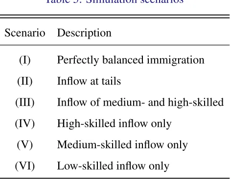
Migration scenarios

Similarly to Felbermayr and Kohler(2007), we simulate migration scenarios for

Table 5: Simulation scenarios

Scenario Description

(I) Perfectly balanced immigration

(II) Inflow at tails

(III) Inflow of medium- and high-skilled

(IV) High-skilled inflow only

(V) Medium-skilled inflow only

(VI) Low-skilled inflow only

In scenario (I), we assume a proportional increase in all skill levels which resembles

approximately the Dutch immigration scenario, see Muysken and Ziesemer (2011). In

scenario (II) we assume immigration to be composed of 75% low-skilled and 25%

high-skilled labour. As pointed out by Felbermayr and Kohler(2007), this denotes the most

realistic case for the past in the OECD countries, as it features bimodality in migration

flows with a bias towards low-skilled migration. We also simulate the model for the

cur-rent migration pattern within the EU (scenario (III)) where the majority of migrants from

new member states (Poland and Baltic states) are predominantly young with medium- or

high skill levels (Blanchflower et al., 2007). In doing so, we use as a benchmark the

rel-ative share of high-skilled foreign labour force in the U.S. which can be seen as a target

value and subtract from that the value for Germany.16 We, then, compute the percentage

inflows such that the overall size of inflows equals 10% of the total labour force.17 The

resulting inflow consists for 44.3% of high skilled workers and the remaining part, 55.7%,

is medium skilled. We also assess the quantitative impact of each skill groups separately

in the scenarios (IV)-(VI). Furthermore, to ensure comparability between the different

cases and due to the fact that just under 10% of the German workforce are foreign born,

all scenarios are specified such that the overall size of the inflow is approximately 10%

16_{As used in the migration literature, seeZiesemer(2011), we take the Worldbank data on migration} stocks which provide information by educational attainment of immigrants and total labour force. However, theWorldbank data setprovides only information for 1975 to 2000 which we use as a proxy.

of the initial labour force. Finally, we assume a full adjustment of capital stock. Hence,

the results indicate long-run effects.

5.2.

Simulation results

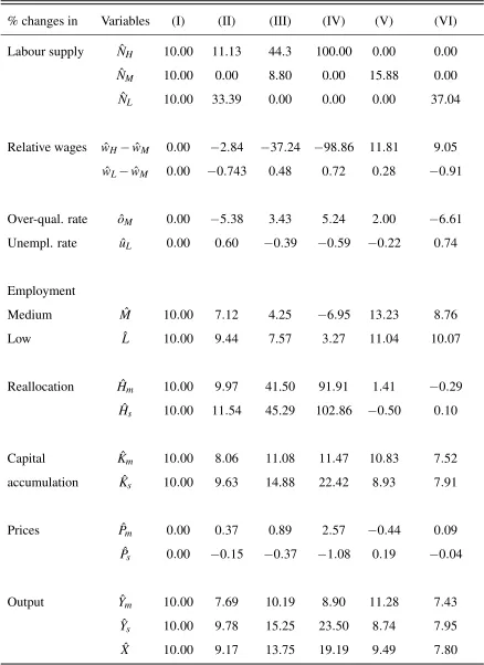
The effect of various migration inflows is shown in Table6. Interestingly, a perfectly bal-anced migration flow has a neutral impact on the receiving economy. This is mainly due

to the linear homogeneity nature of the production functions and full capital adjustments

which verifies the results of the theoretical part (Section4.2.). Migration flow at the tails of the skill distribution (scenario II) has mild positive wage effects for low- and

medium-skilled labour, while high-medium-skilled labour is hurt slightly. The labour market conditions

of medium-skilled workers improve significantly while low-skilled unemployment risk

is increased slightly. Deterioration in the relative commodity prices induces favourable

demand shift for service goods and thus triggers relatively more high-skilled towards that

sector. We see that the one-skill-type migration policy (scenarios (IV)-(VI)) reflect

per-fectly the predictions of the model discussed in the theoretical part. Therefore, changes in

commodity prices (Pm,Ps) due to changes in factor prices (wH,wM,wL) have significant

effects on the reallocation of the mobile labour and on the labour market outcomes of

the sector-specific labour. Looking at the welfare effects by means of GDP per head, we

obtain the widely observed results where high-skilled migration (scenario IV) is

unam-biguously beneficial for the receiving country reflected in an increase of GDP per capita

by 9% whereas low-skilled migration (scenario VI) might indeed be harmful, a decline of

GDP per capita by 2%. However, with respect to medium-skilled migration (scenario V),

the result implies a neutral impact as denoted by the overall increase of GDP per capita by

almost 10%. Moreover, the impact on the relative medium-skilled wage rate shows the

polarization effect confirming our hypothesis that the rise in medium-skilled migration

might partly explain this phenomenon.

Finally, the most plausible scenario of a migration flow at the higher skill distribution

(scenario III), which is dominated by medium skilled workers, has a positive welfare

effect as per capita income rises by 3.75%. This induces us to conclude that overall

Table 6: Simulation of labour market effects of migration

% changes in Variables (I) (II) (III) (IV) (V) (VI)

Labour supply NˆH 10.00 11.13 44.3 100.00 0.00 0.00

ˆ

NM 10.00 0.00 8.80 0.00 15.88 0.00

ˆ

NL 10.00 33.39 0.00 0.00 0.00 37.04

Relative wages wˆH−wˆM 0.00 −2.84 −37.24 −98.86 11.81 9.05

ˆ

wL−wˆM 0.00 −0.743 0.48 0.72 0.28 −0.91

Over-qual. rate oˆM 0.00 −5.38 3.43 5.24 2.00 −6.61

Unempl. rate uˆL 0.00 0.60 −0.39 −0.59 −0.22 0.74

Employment

Medium Mˆ 10.00 7.12 4.25 −6.95 13.23 8.76

Low Lˆ 10.00 9.44 7.57 3.27 11.04 10.07

Reallocation Hˆm 10.00 9.97 41.50 91.91 1.41 −0.29

ˆ

Hs 10.00 11.54 45.29 102.86 −0.50 0.10

Capital Kˆm 10.00 8.06 11.08 11.47 10.83 7.52

accumulation Kˆs 10.00 9.63 14.88 22.42 8.93 7.91

Prices Pˆm 0.00 0.37 0.89 2.57 −0.44 0.09

ˆ

Ps 0.00 −0.15 −0.37 −1.08 0.19 −0.04

Output Yˆm 10.00 7.69 10.19 8.90 11.28 7.43

ˆ

Ys 10.00 9.78 15.25 23.50 8.74 7.95

ˆ

X 10.00 9.17 13.75 19.19 9.49 7.80

6.

Concluding remarks

In this paper we present a theoretical model motivated by our stylized facts with two

major (manufacturing and services) sectors and heterogeneous labour markets defined

by three skill groups to analyse the impact of various skill compositions of immigration.

Particular attention is paid to the impact of immigration of medium skilled workers.

Al-though this has been neglected in the literature, our stylized facts show the importance

of this specific skill group. The analytical solution of the model shows that it is able

to reproduce the stylized facts. We elaborate the labour market as well as the welfare

impacts of different migration scenarios. The following outcomes are at the core of our

analysis. First, a perfectly balanced immigration flow has a neutral effect on the

re-ceiving economy such that GDP per capita remains constant. Regarding the effect of

different skill compositions of immigrants two types of immigration scenarios (skilled

and unskilled) have been extensively studied. In line with the common conclusion we

also find that high-skilled immigration is beneficial for the receiving economy, whereas

low-skilled immigration is harmful. Our main results, which focus on medium skilled

immigration, are complementary to these findings. First, a stronger wage indexation

be-tween medium-skilled and low-skilled might indeed explain the recent negative relation

between the over-qualification rate and the unemployment rate. Second, our framework

indicates that the recent wage polarization effect might be partly explained by the relative

increase in the supply of medium-skilled labour.

Using data for Germany, we analyse the quantitative impact of different

immigra-tion scenarios. The results reveal, indeed, that immigraimmigra-tion of medium-skilled labour

can generate favourable economic outcomes. It boosts, in particular, the labour market

conditions for low-skilled labour. An increase in the medium-skilled endowments raises

total output to the increase of the labour force, indicating a neutral impact. Moreover,

simulating the recent migration pattern (medium- and high-skilled) in the course of EU

enlargement reveals an improvement by 3.75% in per capita income. Second, while the

impact of immigration on unemployment and on over-qualification has been separately

analysed, this paper elaborates the immigration effect on both types of labour market

frictions simultaneously.

Our numerical results also reveal that sector-specific migration induces a

of that sector. Contrary to standard specific-factors models with Walrasian labour

mar-kets where increase in the endowments of the sector-specific factor leads to a contraction

of the other sector due to the reallocation of the mobile factor, we observe that in any

migration scenarios both sectors always expand. The reasoning for this result is that

now immigration of any sector-specific labour has also an adverse effect on the wages of

the other sector-specific labour, an outcome which is essentially due to the wage setting

mechanism resulting from our bargaining model. This induces firms to utilize the

previ-ously idle labour in response to the reallocation of the high-skilled labour into the other

sector.

Furthermore, the endogenous goods prices resulting from the price-setting behaviour

are the important economic mechanism in explaining the substitutability between

differ-ent type of labour. Our findings reveal that labour migration has a productivity effect for

the firms by lowering the production costs. This in turn explains the changes in the skill

intensity across the sectors which in the case of the Cobb-Douglas technology is

essen-tially determined by the relative high-skilled cost shares across the sectors. Moreover,

the neutral impact of medium-skilled migration gives an important insight for policy

de-sign regarding migration policies to satisfy the future labour replacement demand, for

instance, due to ageing.

Appendix: Benchmark statistics and calibration

In order to provide a numerical solution of the model, we match the theoretical model

with the data for a certain period. In doing so, we define values for the production side

such as the input shares as well as for variables and parameters of our designed labour

market like unemployment and over-qualification rates. Our exogenous parameters are

(α,β,ν,η,σx,θ,κ,ξ,δm,δs,λm,λs). The endogenous variables are(Hm,Hs,M,L,uL,oM,

wH,wM,wL,l,h,Ym,Ys,Pm,Ps)with the following exogenous variables(NH,NM,NL). We

compute the values mostly from the EUKLEMS database.18 We also use when necessary

different sources to obtain the values for the specific labour market parameters and

vari-ables. Table7provides an overview of the calibrated and benchmark equilibrium values. Note, in order to have the best-fit of the model with the data, we define the cost shares of

the specific input factors simply as the sum of low- and med-skilled workers cost shares

in each sector. Table8summarizes further the labour market benchmark values.

Table 7: Calibrated and benchmark equilibrium values for the industries

Description Parameter/Variable Value

Manuf. value-add (in 1000 Euros)(a) PmYm 583,191

Service value-add (in 1000 Euros)(a) PsYs 1,393,790

High-skilled labour force (in 1000 persons)(a) NH 3870

Med-skilled labour force (in 1000 persons)(a) NM 24043

Low-skilled labour force (in 1000 persons)(a) NL 10092

Total labour force N=NH+NM+NL 38005

Unemployment rate(b) uL 0.156

Manuf. capital cost share(a) ν 0.27

Manuf. high-skilled cost share(a) α 0.11

Manuf. med-skilled cost share(a) 1−α−ν 0.62

Serv. capital cost share(a) η 0.38

Serv. high-skilled cost share(a) β 0.13

Serv. low-skilled cost share(a) 1−β−η 0.49

Elasticity of Substitution(c) θ = ₁₋1_σx 4

σx 0.75

(a) Computed from EUKLEMS data base.

(b) FromOECD(2007, Table II.A1.1), denoting 2003-2004 average.

Table 8: Labour market benchmark values

Description Parameter/Variable Value

Over-qualification rate(d) oM 0.57

Manuf. high-skilled empl. (in 1000)(e) Hm 1012

Serv. high-skilled empl. (in 1000) Hs=NH−Hm 2859

h= Hm

NH 0.26

Med-skilled empl. (in 1000) M= (1−oM)NM 10339

Low-skilled empl. (in 1000) L= (1−uL)NL+oMNM 22223

l= (1−uL)NL/L 0.38

High-skilled wage rate(f) wH =αPmYm/Hm 63.38

Med-skilled wage rate(f) wM = (1−α−ν)PmYm/M 34.97

Low-skilled wage rate(f) wL = (1−β−η)PsYs/L 30.73

Manuf. trade union bargaining power(g) δm 0.137

λm 0.0743

Serv. trade union bargaining power(h) δs 0.087

λs 0.0658

Proportionate factor(i) ξ 0.565

Weighting factor(j) κ 0.50

Manuf. wage curve _Φ(·) = wM

wL 1.14

Service wage curve _Ψ(·) = wL

wM 0.88

Elasticity manuf. wage curve εoM =−

∂logΦ(·)

∂logoM =−

λm 1+λm

1

oMΦ(·) -0.14

Elasticity serv. wage curve εuL=−

∂logΨ(·)

∂loguL =−

λs 1+λs

1

ξ κuLΨ(·) -1.23

(d) Calibrated to ensurewH>wM>wL>b. (e) Calibration is based on the conditionαPmYm

Hm =wH=β

PsYs

NH−Hm.

(f) Calibration is based on the EUKLEMS data.

(g) Calibrated from the manufacturing wage-setting curve (18) and (15a).

(h) Calibrated from the manufacturing wage-setting curve (22) and (15b).

(i) Assumed.