Analysis of missing values in simultaneous linear functional relationship model for circular variables

Analysis of missing values in simultaneous

linear

functional relationship model for circular variables

S. F. Hassan, Y. Z. Zubairi and A. G. Hussin*

Centre for Foundation Studies in Science, University of Malaya,

50603 Kuala Lumpur, Malaysia.

Circular data is rather special and it cannot be treated just like linear data.

Hence, all existing procedures that have been used in treating the missing

values in linear data are not longer available for circular data. Imputation

methods for missing values data are proposed in the paper. Two different

methods namely circular mean by column and sample mean are used. For

this study, missing values were tested in parameter estimation for

simultaneous linear functional relationship model for circular variables. Via

simulation studies, it shows that the proposed method provide an adequate

approach in handling missing values for circular variables.

Keywords: circular data, circular mean, missing value, simultaneous linear

functional relationship model

*Corresponding author. E-mail: ghapor@um.edu.my

INTRODUCTION

Missing values arise in many research fields and it is a common problem in data

analysis. The missing values can be classified as missing by definition of the

subpopulation, missing completely at random (MCAR), missing at random (MAR), and

nonignorable (NI) missing values.

In view of its common occurrence in data collection, many studies have been

carried out on how to handle the data set with missing values for linear data. Many

approaches have been developed in addressing missing values which can be classified

as the traditional and modern approaches (Acock 2005). Traditional approaches include

listwise deletion, pairwise deletion and replacement procedures. On the other hand,

several modern approaches are applied where some of them are integrated from

traditional approach. Imputation is one of modern approach and it is a class of methods

by which estimation of the missing value or of its distribution is used to generate

predictions from a given model (Tsechansky & Provost 2007).

By far, the most common way to handle missing values is by deleting those

observations with missing values thus leading to a complete analysis. However, this

approach decreases the sample size of data and at the same time will reduce the power

of statistics which in turn, results in biased estimates when the excluded group is a

selective subsample from the study population (Barzi & Woodward 2004). Therefore, a

more pragmatic approach in handling missing values is by using the replacement

procedure. Replacement procedure (Tsikriktis 2005) includes mean substitution,

values are replaced with the mean of available observations. In the other cases, the

missing values can be replaced by mean of subgroup of which the observed values are a member.

Another aspect that needs to be considered when handling the problem of

missing values apart from the types of missing values, is the sample size of data. As

mentioned earlier, deletion approach results in a decrease of sample size and the

statistical power. The imputation approach seems to be a more pragmatic approach.

Nevertheless, the issue of biasness should be taken into account in the imputation

method.

To date, there is no work have been done on missing value for circular data. This

could very well be due to the complexity of the circular data itself and the limited

statistical software available to analyse such data. In the following section, two methods

of data imputation for circular variables are proposed. The imputation methods that are

propose are based on the measure of central location where the circular mean

substitution is used in this analysis. As analogue to linear data, the use of mean

substitution may be based on the fact that the mean is a reasonable guess of a value

for a randomly selected observation from a normal distribution (Acock 2005). In this

study, the evaluations of the proposed methods were assessed using simulation studies

and illustrated using the wind direction data.

THE MODEL

The study of missing values was applied in the simultaneous linear functional

relationship model for circular variables. This model is an extension of the linear

functional relationship model for circular variables which was first introduced by Hussin

(1997). The details of the model can be defined as follows. Suppose the circular

variables ~

(j

=

1,... ,

q)

are related to

X

by the linear relationship

Y

j

=

a

j

+

PjX,

Let

(X;, YjJ

be the true values of the circular variables

X

and

Yj

respectively. The

observations

X;

and

Yji

have been measured with errors

5;

and

5j;

which are

independently distributed with von Mises distribution with mean direction zero and

concentration parameter

K

and

Vj

respectively that is,

5; ~

VM(O,

K)

and

5j; ~

VM(O,

vJ.

Thus the full model can be written as

X; =X;

+

5;

and

Yji =~;

+

5j;,

where

YJ.=

a.

+

pX(mod2;r),

for

j =1,... ,q

) ) .

When

q

=

1, the model is known as linear functional relationship model for circular

variables which have been discussed by Hussin (2003) and Caries and Wyatt (2003).

The maximum likelihood estimate (MLE) of parameters are given as follows;

(i) MLE for

a

j

a)

=

tan

-I { ~ }

+

;r

C

<

°

tan

-I { ~}

+

2;r

S

<

0, C

>

°

where S

=

Lsin&j; - PiX;)

and C

=

L cos&j; - PjX;).

i i

(ii)

MLE for

P

j

~

(iii) MLE for

X;

~ ~

where Xii is an improvement of XjO •

(iv) MLE for

K

Estimation of

K

can be obtained by using the approximation given by Fisher (1993),

2W+W3 +2w5

6

A-l(W)=

-0.4+

1.39w+

(0.43)

l-w

1

w<0.53

0.53 ~

w<

0.85

w~0.85

-«

1:

_.

~

en

a:

>

-,.

::>

z

«

~ ~

CI)

:::>

PROPOSED DATA IMPUTATION OF MISSING VALUES

This section proposed two methods in imputing values for the missing values.

Circular Mean

by

Column

The imputation procedures using circular mean by column implies that for each

column, the circular mean value for each column is evaluated. The column mean is then

used to replace any missing values for the respective columns.

Sample Circular Mean

Another imputation procedure that is proposed in the study is to consider sample

circular mean to impute into the missing values. The sample circular mean is the mean

of the whole dataset excluding the missing values.

SIMULATION STUDIES

The simulation studies were carried out in order to evaluate the performance for "t'

each proposed method. For this purpose, programmes are written using S-Plus. The

simulation studies are repeated for 5000 times and the values of

X

have been drawn

from X""VM

c..

3)

and without loss of generality, the values of aj

=

0

and

P

j

=

1. for

j = 1,2are chosen. Hence the proposed model in this simulations is given by

w

Two different choices of concentration parameters K = 30 and 50 for random error by

assuming 1(.=Vj with sample size n = 100 are considered. The values of It cover a

more realistic range as it is expected the random error of circular variable is less

dispersed. For each sample, we randomly assign 5%, 10%, 15%, 20%, 40% and 50%

of the missing values, respectively.

In these simulation studies, all parameters, a1, a2, /11'

/1

2and K are calculated. As

for performance indicator purposes, the circular mean and circular distance (d) were

calculated for a1 and a2 since these two parameters are in circular form. For parameters

P

1,

P2

and 11:, the mean, estimate bias (EB), and estimate root mean square error

(ERMSE) were calculated as follows.

Calculation for aj where j

=

1..2

i. Circular Mean,

tan"" (~) S>

o.c

>

0

Ii;;;

tan-1 (~)

+

1r C

<

0

tan-1 (~)

+

2x- S

<

o,e

>

0

ii. Circular Distance,

d

=1r

-l1f -

Ia- -

a

II

Calculation for

P

j and 1(where j =1,2

i.

M

_{ean ...}:;:=:; 11; ...

= - ...

-f S J

ii. Estimated Bias, If8=

!~-

wJ

iii. Estimated Root Mean Square Errors, ERMSE =j;l;(1Zj-

wt

All biases were calculated based on the corresponding true value that were used

in generating the data set and between the new estimated values for the data set with

imputed values and labelled as aT. The biases were also calculated based on the

comparison between the initial parameter which has been estimated by simultaneous

linear functional relationship model for circular variables and the new parameters with

imputed values and labelled as

a

j. The following tables show the results obtained from the simulation studies. Method 1 refers to circular mean by column while Method 2

refers to sample circular mean.

Tables 1 and 2 show the simulation results obtained for 1( = 30 using both of the

proposed methods. The results show that the new means are close to the initial

parameters estimated using the simultaneous linear functional relationship model for

circular variables as well as the true value if the percentages of missing values are

smaller such as 5%, 10%, 15% and 20%. However, the new means suddenly diverged

quite far from the initial parameter once the percentage of missing values increased

beyond 20%. In other words, if the percentage of missing values is too high, for

example if the percentage of missing values reaches to at least 40%, the estimation

seems to diverge from the initial value and produces high value of estimate bias. Thus,

it can be inferred that when the percentage of missing values reach more than 40%, the

Table 1: Simulation results for a1and az using proposed methods for l( =30

Parameter CIl Cl:l

True Value 0.0000 0.0000

Estimated Value 6.2708 6.2773

Performance

Parameter Percentage Method 1 Method 2 Method 1 Method 2 Indicator

5% 6.2660 6.2661 6.2697 6.2703

10% 6.2621 6.2639 6.2667 6.2693

Mean 15% 6.2589 6.2621 6.2630 6.2659

20% 6.2564 6.2602 6.2621 6.2654

40% 6.2476 6.2518 6.2548 6.2570

50% 6.2407 6.2489 6.2446 6.2520

5% 0.0047 0.0047 0.0075 0.0070

10% 0.0087 0.0069 0.0105 0.0079

.... 15% 0.0119 0.0087 0.0142 0.0113

'*j

20% 0.0143 0.0106 0.0151 0.0119

40% 0.0231 0.0190 0.0225 0.0202

Circular 50% 0.0301 0.0219 0.0327 0.0252

Distance, d 5% 0.0171 0.0171 0.0135 0.0129

10% 0.0211 0.0193 0.0164 0.0139

15% 0.0243 0.0211 0.0202 0.0173

Cl"

20% 0.0267 0.0230 0.0211 0.0178

40% 0.0356 0.0314 0.0284 0.0261

50% 0.0425 0.0343 0.0386 0.0311

From Table 1, the values of circular distance (d) for a1 and az which correspond

to true value (aT) are higher than the values which correspond to the initial parameter

estimate (ilj). It shows that the new mean with imputed values are closer to the initial

parameter estimated rather than the true value used in generating the data itself. This is

not suprise as the generated data with imputations are quite similar to the generated

data itself.

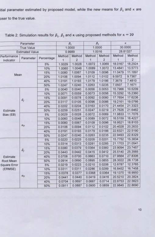
From Table 2, it can be seen that the estimate bias between the new imputed

values with initial parameter estimated are smaller for

112

while for

P

1and K,the estimate

bias between the new imputed values and true value are smaller than the bias between

and initial one. Therefore, it can be concluded that the new mean for

P2

is closer to

initial parameter estimated by proposed model, while the new means for

Pl.

and 1(. are

[image:10.532.15.523.44.821.2]

closer to the true value.

Table 2: Simulation results for

P

l,

P

2 and K using proposed methods for K =30

Parameter

"1

P1.

i'C

True Value 1.0000 1.0000 30.0000

Estimated Value 0.9989 1.0016 28.81327

Performance

Parameter Percentage Method Method Method Method Method Method

Indicator 1 2 1 2 1 2

5% 1.0029 1.0028 1.0072 1.0069 18.0167 18.2924 10% 1.0060 1.0048 1.0089 1.0072 13.4841 13.5773

Mean 15% 1.0080 1.0067 1.0109 1.0096 11.0479

11.1897 20% 1.0106 1.0094 1.0112 1.0102 9.5972 9.7367 40% 1.0191 1.0193 1.0179 1.0186 7.3679 7.4810 50% 1.0247 1.0240 1.0263 1.0235 7.0507 7.1671 5% 0.0040 0.0040 0.0056 0.0053 10.7966 10.5209 10% 0.0071 0.0059 0.0073 0.0056 15.3292 15.2360

at

_20%15% 0.0091_0.0117 0.0078_0.0105 0.0092_0.0096 0.0080_0.0086 17.7654_19.2161 17.6236_19.0766 40% 0.0202 0.0204 0.0163 0.0170 21.4454 21.3323 Estimate 50% 0.0259 0.0251 0.0247 0.0219 21.7626 21.6462 Bias (EB) 5% 0.0029 0.0028 0.0072 0.0069 11.9833 11.7076 10% 0.0060 0.0048 0.0089 0.0072 16.5159 16.4227 15% 0.0080 0.0067 0.0109 0.0096 18.9521 18.8103

aT

20% 0.0106 0.0094 0.0112 0.0102 20.4028 20.2633 40% 0.0191 0.0193 0.0179 0.0186 22.6321 22.5190 50% 0.0247 0.0240 0.0263 0.0235 22.9493 22.8329 5% 0.0220 0.0225 0.0205 0.0201 15.7752 15.3834 10% 0.0314 0.0313 0.0281 0.0285 21.1703 21.0541

A 15% 0.0380 0.0379 0.0364 0.0360 23.9094 23.7457

af

20% 0.0443 0.0442 0.0415 0.0412 25.5140 25.3565 Estimate 40% 0.0708 0.0700 0.0663 0.0710 27.9564 27.8306 Root Mean 50% 0.0914 0.0890 0.0895 0.0855 28.3022 28.1738 Square Error 5% 0.0219 0.0223 0.0210 0.0206 12.6787 12.3765 (ERMSE) 10% 0.0311 0.0311 0.0286 0.0289 16.8452 16.7458 15% 0.0378 0.0377 0.0368 0.0364 19.1370 18.9950

aT

Table 3: Simulation results for a1and az using proposed methods for J( =50

Parameter at a~

True Value 0.0000 0.0000

Estimated Value 6.2790 6.2366

Performance

Parameter Percentage Method 1 Method 2 Method 1 Method 2 Indicator

5% 6.2750 6.2757 6.2347 6.2362

10% 6.2724 6.2713 6.2326 6.2365

Mean 15% 6.2691 6.2696

6.2326 6.2366

20% 6.2684 6.2673 6.2316 6.2362

40% 6.2615 6.2616 6.2264 6.2364

50% 6.2598 6.2576 6.2244 6.2367

5% 0.0040 0.0033 0.0019 0.0005

10% 0.0066 0.0077 0.0040 0.0002

,_ 15% 0.0099 0.0094 0.0040 0.0000

rIj

20% 0.0106 0.0117 0.0050 0.0004

40% 0.0175 0.0174 0.0102 0.0003

Circular 50% 0.0192 0.0214 0.0122 0.0001

Distance, d 5% 0.0082 0.0075 0.0484 0.0470

10% 0.0108 0.0119 0.0505 0.0467

15% 0.0141 0.0136 0.0506 0.0466

aT'

20% 0.0147 0.0159 0.0515 0.0470

40% 0.0216 0.0216 0.0568 0.0468

. 50% 0.0234 0.0256 0.0588 0.0465

Tables 3 and 4 show the simulation results for JC =50 using both of the proposed

methods. The results also seems to exhibit the same pattern as for JC = 30, where the

mean values are close to the initial parameter estimated as well as the true parameter

used in generated the data. The value of estimate bias (EB) and estimate root mean

square error (ERMSE) also increases as the percentage of missing values increases to

at least 40%.

The new mean is closer to the initial parameter estimated as well as to the true

parameter, but the increment in the percentage of missing values being imputed using

the proposed method has led to high divergence of new mean as well as having large

value of estimate bias and estimate root mean square error.

Table 4: Simulation results for

Pi'

P

2 and K proposed methods for K =50

Parameter

Pr.

P:2 I(;

True Value 1.0000 1.0000 50.0000

Estimated Value 0.9954 1.0167 47.7866

Performance

Parameter Percentage Method Method Method

Method Method Method

Indicator 1 2 1 2 1 2

5% 0.9984 0.9979 1.0184 1.0184 27.7332 27.9003 10% 1.0002 1.0015 1.0199 1.0190 20.2977 20.4992

Mean 15% 1.0039

1.0033 1.0210 1.0203 16.5384 16.7316 20% 1.0057 1.0058 1.0225 1.0214 14.3439 14.4662 40% 1.0116 1.0120 1.0284 1.0266 10.7750 10.8732 50% 1.0172 1.0183 1.0345 1.0311 10.2543 10.2923 5% 0.0030 0.0025 0.0017 0.0016 20.0534 19.8863 10% 0.0048 0.0061 0.0032 0.0023 27.4889 27.2874

fij 15% 0.0085

0.0079 0.0042 0.0036 31.2482 31.0550 20% 0.0103 0.0105 0.0058 0.0047 33.4427 33.3204 40% 0.0162 0.0166 0.0117 0.0099 37.0116 36.9134 Estimate

50% 0.0218 0.0229 0.0177 0.0143 37.5323 37.4943

Bias (EB) 5%

-

-0.0016 0.0021 0.0184 0.0184 22.2668 22.0997 10% 0.0002 0.0015 0.0199 0.0190 29.7023 29.5008

aT 15% 0.0039 0.0033 0.0210 0.0203 33.4616 33.2684 20% 0.0057 0.0058 0.0225 0.0214 35.6561 35.5338 40% 0.0116 0.0120 0.0284 0.0266 39.2250 39.1268 50% 0.0172 0.0183 0.0345 0.0311 39.7457 39.7077 5% 0.0187 0.0187 0.0176 0.0178 28.3970 28.1876 10% 0.0269 0.0270 0.0253 0.0251 37.2483 37.0155

,"" 15% 0.0337 0.0329 0.0299 0.0305 41.5185

41.3005

CLj

20% 0.0386 0.0385 0.0353 0.0349 43.9727 43.8359 Estimate 40% 0.0561 0.0560 0.0525 0.0525 47.9229 47.8148 Root Mean 50% 0.0665 0.0681 0.0639 0.0631 48.4952 48.4530 Square Error 5% 0.0185 0.0186 0.0255 0.0255 22.6922 22.5315 (ERMSE) 10% 0.0265 0.0263 0.0321 0.0314 29.8666 29.6691 15% 0.0329 0.0321 0.0363 0.0365 33.5447 33.3541

aT

20% 0.0376 0.0375 0.0415 0.0407 35.7052 35.5838 40% 0.0550 0.0548 0.0586 0.0581 39.2425 39.1447 50% 0.0651 0.0667 0.0704 0.0689 39.7602 39.7218

Based on the simulation studies using different concentration parameters namely

K

=

30 and 50, by imputing values for missing observations in the data, the estimated

value of the new mean seems to provide a good estimate. This can be seen by small

of the value of concentration parameter, the parameter estimation has small bias so

long as the percentage of missing values at most 20%. On the other hand, if the

percentages of missing values reach at least 40%, the estimates produced from the

data set seem inadequate. This can be seen in the high values of biases and can be

said to be not acceptable. In short, we can say that if the percentage of missing values

in our data is less than or equal to 20%, the analysis can be performed using the

proposed methods.

Comparison between both proposed methods also can be made to determine

which of the two methods perform better. From the simulation results, it can be seen

that the Method 2 which is sample circular mean is a more superior approach. Based on

the values of estimate bias and estimate root mean square error for each method, it can

be seen that the second method, sample circular mean, gives a relatively small bias in

comparison to the first method, that is, the circular mean by column. This implies that

the second method give better estimate in comparison to the first method. The second

method uses the approach where it considers the circular mean for the whole data set

which excludes all missing values.

From Tables 1 to 4, it can be seen that the estimate bias of concentration

parameter, l( gets larger and larger as the value of lC increases. Hence, it can be said

that as the concentration parameter of random error increases, the estimation of K. in

analyzing the missing values gives high value of estimate bias as well as their estimate

root mean square error. Hence, it can be said that apart from the increase in the

percentage of missing values, the increase in value of concentration parameter K. also

leads to the increase in biasness for parameter K.

ILLUSTRATION USING REAL DATA SET

As an illustration for the proposed method, the real data set which is the wind

direction data collected at three different levels so that it suits in the prior model,

namely, simultaneous linear functional relationship model for circular variables was

used. The dataset was recorded at Sayan Lepas airport which is located at Penang

Island, north of Malaysia. The measurements was taken on July and August 2005 at

time 1200, located at 16.3 m above ground level, latitude 05°18'N and longitude

100016'E. A total of 62 observations have been recorded at three different pressures

with their corresponding height as follows:

i. at pressure 850 Hpa with 5000 m height as variable

x

ii. at pressure 1000 Hpa with 300 m height as variable

Y1

iii. at pressure 500 Hpa with 19000 m height as variable

Y2

Table 5: Results for

"1

and a2 for Sayan Lepas

Parameter IZl a2;

Estimated Value -0.2108 -0.1740

Performance

Percentage Method 1 Method 2 Method 1 Method 2 Indicator

5% 0.0867 0.0437 0.1899 0.1580

10% 0.1807 -0.0924 0.2008 0.1485

Mean 15% 0.2449 -0.2886 0.1591 0.1403

20% 0.2148 -0.4865 0.0574 0.1102

40% -0.2390 -1.1881 -0.2521 0.1005

50% -0.3749 -1.3684 -0.3895 0.0859

5% 0.2975 0.2545 0.3639 0.3320

10% 0.3915 0.1183 0.3748 0.3225

Circular 15% 0.4556 0.0778 0.3331 0.3143

Distance, d 20% 0.4256 0.2758 0.2314 0.2842

40% 0.0283 0.9774 0.0781 0.2745

Table 6: Results for /11'

P2

and K for 8ayan Lepas

Parameter _fin

_P'l

_'"

Estimated Value 1.0340 0.9119 1.0259

Performance

Percentage Method 1 Method 2 Method 1 Method 2 Method 1 Method 2 Indicator

5% 0.9124 0.9643 0.8425 0.8830 1.0192 1.0205 10% 0.8316 0.8953 0.8156 0.8986 1.0365 1.0423

Mean 15% 0.7424 0.8401 0.8066 0.9234

1.0679 1.0721 20% 0.6907 0.7793 0.8201 0.9614 1.0991 1.1074 40% 0.4902 0.7447 0.8820 1.1525 1.2923 1.3232 50% 0.4802 0.7799 0.9215 1.2152 1.3894 1.4351 5% 0.1216 0.0698 0.0693 0.0288 0.0067 0.0054 10% 0.2024 0.1387 0.0963 0.0132 0.0106 0.0164 Estimate 15% 0.2916 0.1939 0.1053 0.0116 0.0420 0.0462 Bias (EB) 20% 0.3433 0.2547 0.0917 0.0495 0.0731 0.0815 40% 0.5438 0.2893 0.0299 0.2407 0.2663 0.2973 50% 0.5538 0.2541 0.0096 0.3033 0.3635 0.4092 5% 0.2722 0.1580 0.1161 0.1244 2.0187 2.0198 Estimate 10% 0.4110 0.2781 0.1756 0.1774 2.0337 2.0387 Root Mean 15% 0.5255 0.3492 0.2141 0.2515 2.0606 2.0643 Square Error 20% 0.5941 0.4241 0.2462 0.3218 2.0874 2.0947 (ERMSE) 40% 0.7836 0.4901 0.3546 0.6980 2.2566 2.2842 50% 0.7985 0.4707 0.3729 0.8147 2.3430 2.3845

Tables 5 and 6 show the results obtained from the analysis for the real

data sets using the proposed methods as describe earlier. From the results obtained, it

gives a similar trend as in the simulation studies where it can be seen that the estimates

are quite good for small percentages of missing values. The increment in percentage of

missing values leads to the increment in all biases. In particular, if the percentages of

missing values reach to 40% or higher, we can say that analyses give poor estimates

and this can be seen from the large value of biases.

Consistent with the findings in the simulation studies, Tables 4 and 5 show that

Method 2 gives relatively small value of circular distance,

d

in comparison to Method 1.

This implies that Method 2 gives better estimation for a1 and a2;. The similar results also

can be seen for parameter

P1

and

pz

where Method 2 give the better estimation

compared to Method 1 based on the value of estimate bias and their estimate root

mean square error for each parameter. The estimation of K are consistent as the

simulation study where high value of concentration parameter will give a higher value of

estimate bias and their estimate root mean square error.

DISCUSSION

In this paper, a more in-depth study on parameter estimation using simultaneous

linear functional relationship model for circular variables was carried out. In the analysis,

data sets consisting of three circular variables, specifically called as three different

levels were used. The data set consisted of three columns where each column

represented each circular variable. Two imputation methods were proposed for missing

values in the data set known as circular mean by column and sample circular mean.

Circular mean by column will consider mean for each column after excluding all missing

values, while sample circular mean treats all observations in number of columns as

whole data sets. Finally the circular mean will be evaluated after excluding all missing

values.

From the simulation study, it can be shown that Method 2, namely, sample

circular mean is more superior in comparison to Method 1. This is based on the

comparison of all performance indicators which are circular distance (d), estimate bias

(ES) and estimate root mean square error (ERMSE). It can be summarized the

smaller i.e at most 20%. At the same time, it can be seen that all biases also increased

as the percentage of missing values increased and this has led to inconsistent

estimation.

The findings are consistent by varying the values of concentration parameter.

Therefore, it can be concluded that with presence of missing variables, it can be

overcome by imputing the missing values with circular mean. The estimate obtained has

small bias, thus indicate a good approach in the analysis. Furthermore, as variables are

related to each other, the imputing approach using circular mean uses the information of

central tendency into the data set.

REFERENCES

Acock, A. C. (2005). Working with missing values. ProQuest Education Journals.

Journal of Marriage and Family, 67(4), 1012-1028.

Barzi, F.

&

Woodward, M. (2004). Imputations of missing values in practice: Results

from imputations of serum cholestrol in 28 cohort studies. American Journal of

Epidemiology, 160(1),34-45.

Caries, S. & Wyatt, L. R. (2003). A linear functional relationship model for circular data

with an application to the assessment of ocean wave measurements. Journal of

Agricultural, Biological, and Environmental Statistics, 8(2), 153-169.

Hussin, A. G. (1997). Pseudo-replication in functional relationship with environmental

application. PhD Thesis, School of Mathematics and Statistics, University of

Sheffield, England.

Hussin, A. G. & Chik, Z. (2003). On estimating error concentration parameter for circular

functional model. Bull. Malaysian Math. Sc. Soc., 26, 181-188.

Little, R. J. A. & Rubin, D. B. (1987). Statistical Analysis with Missing Data. New York:

Wiley.

Tsechansky, M. S

&

Provost, F. (2007). Handling missing values when applying

classification models. Journal of Machine Learning Research, 8, 1625-1657.

Tsikriktsis, N. (2005). A review of techniques for treating missing data in OM survey