Comparison of Controller Performance for MIMO Process

(1)

International Journal of Emerging Technology and Advanced Engineering

Website: www.ijetae.com (ISSN 2250-2459, ISO 9001:2008 Certified Journal, Volume 3, Issue 8, August 2013)

51

Comparison of Controller Performance for MIMO Process

Jayaprakash J

1

, Davidson D

2

, Subha Hency Jose P

3

1,2_{PG Scholar Karunya University}

3_{Assistant Professor Karunya University}

Abstract— The main objective of this paper is to simulate

and control some different aspects of multivariable control system of the quadruple tank process. The ideas are illustrated on a quadruple tank process with two inputs and two outputs. The level control for a Quadruple tank process with variable non-linear zero dynamics is considered. The multivariable zero dynamics of the system can be made both minimum and non-minimum phase by simply changing the valve position. The process model has been developed from fundamentals and tuned with experimental data. The quadruple tank process is simulated and various controller responses are compared.

Keywords— Quadruple tank process, multivariable control,

minimum phase, non-minimum phase and Sliding mode control.

I. INTRODUCTION

The control of liquid level in tanks and flow between tanks is a basis problem in process industries. Industries have a huge number of interacting control loops. Most of the large and complex industrial processes are naturally Multi input Multi Output (MIMO) systems. They are more complex to control and a challenging task due to inherent nonlinearity and existence of interactions among input and output variables [1]. Most of the industry faces control problems that they are non-linear and have many manipulated and controlled variables. Multivariable control includes both linear and non-linear design methods.

Quadruple tank process was a new laboratory process that has been designed to illustrate performance limitations due to zero location in multivariable control systems [2]. It is a level control problem based on four interconnected tanks and two pumps. The inputs to the process are the voltage to the pumps and outputs are the water levels in the lower two tanks. Many times the liquid will be processed by chemical or mixing treatment in the tank, but always the level of fluid in the tank must be controlled and the flow between tanks must be regulated. The Quadruple tank was developed in the 1996 at Lund institute of Technology, Sweden in order to illustrate the importance of multivariable zero location for control design [5].

The inputs signals are the voltages u1, u2 applied to the two pumps and the outputs are y1, y2 representing the water level in tanks 1 and 2 respectively. There are two non-linear valves that facilitate flows to the tank. One of the features of the linear dynamic model for the process is the variable zero which can be located in either the Right or Left Half Plane (RHP, LHP) depending on the adjustable valve settings. This provides an interesting challenge for linear design paradigms [3].

Variable structure control systems have gained significant attention in process control systems. Various workers have worked to deepen the roots of sliding mode theory and coupled it. A different kind of design strategies have been discussed in this paper for the above problem.

In this paper a classical decentralized PI control strategy has been implemented. The issues related to sliding mode control implementation on quadruple tank process and present an analysis of sliding mode controller design. The results and responses were compared for all the implemented controllers.

II. QUADRUPLE TANK PROCESS

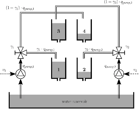
The Quadruple tank process is a laboratory process that consists of four interconnected tanks and two pumps. The schematic diagram of the process is shown in Figure 1

The process inputs are u1 and u2 (input voltages to pumps, (0-10 V)) and the outputs are y1 and y2 (voltages from level measurement devices (0-10V)). The target is to control the level of the lower two tanks with inlet flow rates. The output of each pump is split into two using a three-way valve. Thus each pump output goes to two tanks, one lower and another upper, diagonally opposite and the ratio of the split up is controlled by the position of the valve.

(2)

International Journal of Emerging Technology and Advanced Engineering

[image:2.612.56.279.140.323.2]

52

Figure 1: Layout of the Quadruple tank process

If Ɣ1 is the ratio of the valve for the first tank, then (1-Ɣ1) will be the valve ratio for the fourth tank. The voltage applied to pump is ui and the corresponding flow is kiui. The parameters Ɣ1 Ɣ2 Ƹ [0, 1] are determined from how the valves are set prior to an experiment. The flow to tank 1 is Ɣ1k1u1 and the flow to flow tank 4 is (1-Ɣ1) k1u1 and similarly for tank 2 and tank 3. The acceleration due to gravity is denoted by g. The measured level signals are y1=kch1 and y2=kch2

[2] .

III. MODEL DEVELOPMENT

To investigate how the behavior of a process changes with time under influence of changes in the external disturbances and manipulated variables and to consequently design an appropriate controller is use two different approaches can be implemented. One is experimental and the other is theoretical. In such case a representation of the process is required in order to study its dynamic behavior. This representation is usually given in terms of a set of mathematical equations whose solution gives the dynamic behavior of the process

For each tank i=1…4, consideration of mass balances and Bernoulli’s law yields:

- (1)

Where Ai denotes the cross sectional area of the tank, hi is the water level, is the in-flow of the tank and is

the out-flow of the tank.

√ (2)

Where ai denotes the cross-sectional area of the outlet hole, g is the acceleration due to gravity. Each pump i=1, 2 gives a flow proportional to the control signal as follows:

(3)

Where ki is the pump constant. Considering the flow in and out of all tanks simultaneously, the non-linear dynamics of the quadruple tank process is given by:

√ √

√

√ (4)

The above mass balance and Bernoulli’s law can be re-written as

√ √

√

(5)

The replacement of non-linear model by its linear approximation is called linearization. The linearized dynamics at a given stationary operating point is determined from the state space:

and y=C x (6)

Where

[

_]

,

[

]

(3)

International Journal of Emerging Technology and Advanced Engineering

53

, and represents the time

constants given by √ .

At a particular , the stationary control signal is obtained by solving the following:

_*

+ (8)

Where . It is shown that the system is in

non-minimum phase for 0< and minimum phase for 1< . For this two operating points, we have the following time constants [2]:

TABLE 1 TIME CONSTANTS

P- P+

(T1,T2) (62,90) (63,91) (T3,T4) (23,30) (39,56)

The physical modeling gives the two transfer function matrices:

*

+

*

+ (9)

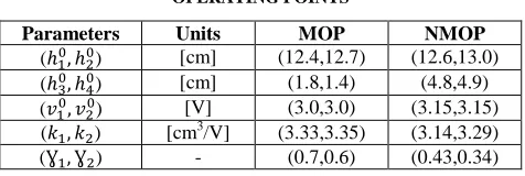
[image:3.612.325.566.158.289.2]

The chosen operating points[2] correspond to the following parameter values are in Table 2:

TABLE 2 OPERATING POINTS

Parameters Units MOP NMOP

( ) [cm] (12.4,12.7) (12.6,13.0) ( ) [cm] (1.8,1.4) (4.8,4.9) ( ) [V] (3.0,3.0) (3.15,3.15) ( ) [cm3/V] (3.33,3.35) (3.14,3.29) ( ) - (0.7,0.6) (0.43,0.34)

[image:3.612.50.288.535.615.2]

The parameter values[2] of the laboratory process are given in the following table 3:

TABLE 3 PARAMETER VALUES

Parameters Units Values

A1, A3 [cm2] 28

A2, A4 [cm2] 32

a1, a3 [cm2] 0.071

a2, a4 [cm 2

] 0.057

kc [V/cm] 0.50

g [cm/s2] 981

IV. MULTI-VARIABLE ZERO LOCATION AND

CALCULATION

The transmission zeros of a multivariable transfer function matrix of s that cause the input-output matrix to lose rank. That is, the transmission zeros are the values of ‘s’ that cause det [G(s)] =0. RHP transmission zeros for a particular transfer function matrix become RHP poles for the inverse transfer function matrix (i.e., inverse is unstable). If a multivariable controller that simply tries to invert the process model then it will make the system unstable.

The zeros of the transfer matrix are the zeros of the numerator polynomial of the rational function [6]:

* +

(10)

The transfer matrix thus has two finite zeros for γ1, γ2 ϵ (0, 1). One of them is always in the left half-plane, but the other can be located either in the left or the right half-plane. This system is non-minimum phase for and minimum phase for [9]. Recall that

for P-, and for P+. The

(4)

International Journal of Emerging Technology and Advanced Engineering

54

The flow to the lower tanks is smaller than the flow to the upper tanks if the system is non-minimum phase. It is easier to control y1 with u1 and y2 with u2, if most of the flows go directly to the lower tanks. The control problem is particularly hard if the total flow going to the left tanks (Tanks 1 and 3) is equal to the total flow going to the right tanks (Tanks 2 and 4). This corresponds to i.e., a multivariable zero in the origin. There is an immediate connection between the zero location of the model and physical intuition of controlling the quadruple-tank process. The scalar systems and multivariable systems can be distinguished by the location of a multivariable zero and its direction. We define the (output) direction of a zero z as a vector Ψ € R2

of unit length such as ΨTG (z) =0. If Ψ is parallel to a unit vector, then the zero is only associated with one output. If this is not the case, then the effect of a right half-plane zero may be distributed between both outputs. For the transfer matrix, the zero direction for z>0 is given by [2]

[ ] *

+ * + (11)

Note that it follows from this equation that ( ) ≠ 0, so the zero is never associated with only one output. If we solve the above equation for and simplify, it is easy to show that [2]

(12)

From the above equation it is possible to conclude that if is small, and then z is mostly associated with the first output. If is close to one, then z is mostly associated with the second output. Hence, for a given zero location, the relative size of and determines to which output the right half-plane zero is related to.

Solve for both minimum and non-minimum

phase transfer functions:

|

| (13)

s1=-0.0164, s2=-0.06039 shows that both the zeros are present in the left-half plane for minimum phase operating points. The matrix inverse will be stable.

|

| (14)

s1=+0.013, s2=-0.056 shows that presence of right-half plane transmission zero for non-minimum phase operating points. The matrix inverse will be unstable.

V. RELATIVE GAIN ARRAY

The relative gain array (RGA) was introduced by Ed Bristol (1966) as a measure of interaction in multivariable control systems. The RGA is defined as , where the asterisk denotes the Schur product (element-by-element matrix multiplication) and -T denotes inverse transpose. It is possible to show that the elements of each row and column of sum up to one, so for a 2 X 2 system the RGA is determined by the scalar . It is used as a

tool in process industry to decide on the control structure issues such as input-output pairing for decentralized PI controller [2].

The system is particularly hard to control if .

(

) (15)

It can be written as

(

)

Where,

From the above expression, we conclude that the RGA is only depending on the valve settings and no other physical parameters of the process. From the RGA analysis, the values are found and the result is discussed below. The RGA for minimum phase is given by and for non-minimum phase . RGA analysis indicates that the non-minimum phase system is harder to control than the minimum phase system.

VI. DECENTRALIZED PICONTROLLER

(5)

International Journal of Emerging Technology and Advanced Engineering

[image:5.612.57.271.142.231.2]

55

Figure 2: Decentralized PI Controller

This is a simplistic approach to control the multivariable system. It is to disregard cross couplings and treat one loop at a time, as if other inputs and outputs did not exist. The controllers are constructed for ui that is based only on the measured signal yj and its set point rj. Such a controller is said to be decentralized. Decentralized controllers are always square: if the number of inputs and outputs are not the same, simply some of the signals are not used. When there is interaction in process, it can be measured using RGA. Only when the diagonal elements of RGA (G (0)) are positive and with the decentralized controller, the process can be controlled. If some diagonal element of RGA (G (0)) is negative and the decentralized controller is used, then either the closed-loop system is unstable or it will become unstable if one of the SISO loops is broken. So, only the minimum phase system can be controlled using decentralized PI controller.

PI Controller is in the form

( ), (16)

Where

is the Proportional gain of controller is the Integral gain of controller

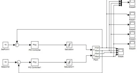
[image:5.612.330.557.145.234.2]

The single loop controllers cannot suppress the interactions of the MIMO process because each input affects not only its corresponding output but also the other ones.

Figure 3: Simulink diagram of Quadruple Tank Process with PI controller

[image:5.612.329.559.259.349.2]

Figure 4: Response of Decentralized PI controller for minimum phase

Figure 5: Response of Decentralized PI controller for non-minimum phase

Figure 3 shows the Simulink diagram of quadruple tank process with PI controller when operated in both minimum and non-minimum phase. Figure 4 and 5 shows the PI response of quadruple tank process. Error of set point and present height is given as input to the controller. The value of PI controller is chosen using the root locus technique. Kp, Ki values of PI controller for Pump 1 is 1.19, 0.01923 respectively. Kp, Ki values of PI controller for pump 2 is 1.607, 0.017 respectively. For these values the tank level settles with their set point given and the responses of the tanks are observed. Here response time for tank 1 and tank 2 is 400sec. Peak over shoot is about 2.7cm and 2.5cm for tank 1 and tank 2 respectively.

PI controller giving poor performance because it takes minimum 400sec to attain the given set point. Generally controller should be very fast. It should give the fast response for all the uncertainties. The over shoot indicates the impact of interaction between the tanks. From the result it is better understood that output of tank 1 and tank 2 takes long settling time. And it is difficult to control the process when operated in non-minimum phase.

VII. SLIDING MODE CONTROLLER

[image:5.612.58.281.573.693.2]

(6)

International Journal of Emerging Technology and Advanced Engineering

56

Sliding mode control (SMC) is a popular approach to control system design under heavy uncertainty, which remains one of the main subjects of modern control theory. SMC is precise, and usually very simple to implement. The main drawbacks of classical first-order Sliding Modes are principally related to the so-called chattering effect. The main cause of chattering has been identified as the presence of un-modeled parasitic dynamics in the switching devices. Advantages of sliding mode controllers are that it is computationally simple compared adaptive controllers with parameter estimation and also robust to parameter variations. The disadvantage of sliding mode control is sudden and large change of control variables during the process which leads to high stress for the system to be controlled. It also leads to chattering of the system states.

The problem is to regulate a dynamic system subject to parameter uncertainties and nonlinearities. A controller is sought to force the system to reach, and subsequently remain on, a predefined surface called the sliding surface with in the state space. The dynamical behavior of the system, when confined to the surface, is called the sliding motion. The advantages of obtaining such motion are twofold; there is a reduction in order; and the sliding motion is insensitive to parameter variations. The latter property of invariance towards uncertainty makes the methodology an attractive one for designing robust control for uncertain systems.

The two components of design approaches are,

1.The design of a sliding surface in the state space, so that the reduced order sliding motion satisfies the specifications imposed on the design.

2.The synthesis of a control law, discontinuous about the sliding surface, such that the trajectories of the closed loop motion are directed towards the surface. The closed loop dynamical behavior obtained for using a variable structure control laws, comprises two distinct types of motion. The initial phase, often referred to as the reaching phase, occurs whilst the states are being driven towards the sliding surface. This motion is, in general, affected by the disturbances present. Only when the states reach the surface, and the sliding motion takes place, does the system become insensitive to uncertainty.

A sliding mode will exist if, in the vicinity of the sliding surface, the state velocity vectors are directed towards the surface. In such a case, the sliding surface attracts trajectories when they are in its vicinity; and it will stay on once a trajectory intersects the sliding surface.

VIII. FEEDBACK LINEARIZATION

Mostly sliding mode controller is used for complex nonlinear MIMO system. In design of sliding mode controller, the feedback linearization technique is used to linearize the nonlinear equation. The central idea of the approach is to algebraically transform a nonlinear system dynamics into a fully or partly linear one.

It can be viewed as ways of transforming original system models into equivalent models of a simpler form. Thus it can also be used in the development of robust nonlinear sliding mode controllers. In simplest form, feedback linearization amounts to canceling the nonlinearities in a nonlinear system so that the closed loop dynamics is in a linear form. When the nonlinear dynamics is not in a controllability canonical form, one may have to use algebraic transformations to first put the dynamics into the controllability form before using the above feedback linearization design. There are two types of partial linearization is available. One is Input State Linearization and second Input Output linearization.

The standard normal form for a 2 2 multiple input and multiple output (MIMO) process model is [7]:

̇

̇ ̈

̇

̇ ̈ (17)

The complete dynamics of the system is represented by state vector

(18)

Output vector is (19)

Superscript used in above model stand for the respective output.

The sliding mode controller output is

* +

( ( √ * (

( γ)

√ *

(_√( γ)* (_√γ * )

(

( _*

(

√

)

(7)

International Journal of Emerging Technology and Advanced Engineering

[image:7.612.328.553.129.261.2]

57

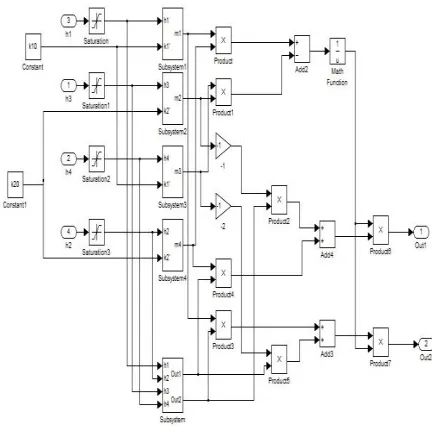
Since level of the tanks of the system keeps on varying, a saturation block is used. Here we are taking inverse in so many places, sometimes water level may be 0. So if we not using saturation the value may be infinitive it collapses all the system. This controller gives the fast response when it is compare with conventional PI controller.

Figure 6: Simulink model of Quadruple Tank Process

[image:7.612.58.278.213.394.2]

Figure 7: Simulink model of Sliding mode controller

Figure 8: Simulink model of Servo response of PI and SMC controller

In the servo response, the setpoint of the plant changes with a particular time. Here for that we are using the Repeating Sequence block to change the setpoint value when simulation is running. Figure 8 shows simulink model of servo response of SMC and PI controller. The setpoint value changes with time, from 0-249sec the setpoint is 15cm, from 250-500sec the setpoint will be 10cm, again from 501-1000sec the setpoint will be 15cm.

Figure 9 and 10 distinguishes the servo response of PI and SMC controller for tank 1 and tank 2. From the Figure it is understood that the SMC controller performs well for set point change than PI controller. For Tank 1 the over shoot value is 0.5cm for SMC and 2.5cm for PI while setting initially. After changing the set point value Peak overshoot is very small for SMC and 0.5cm for PI controller. Tank 2 over shoot value is 0 for SMC and 2.5cm for PI while setting initially. Then after changing set point value Peak overshoot of SMC is 0 and PI is negligible.

[image:7.612.56.272.423.636.2]

(8)

International Journal of Emerging Technology and Advanced Engineering

[image:8.612.55.281.135.361.2] [image:8.612.333.550.226.388.2]

58

Figure 9: Servo responses of SMC and PI for Tank 1 and 2

Figure 10: PI controller output for servo response

Figure 11: Simulink model of Regulatory response of PI and SMC controller

Regulatory response is defined as the response of the controller reaction when any uncertainties occur in the plant side. Uncertainties may be due to sudden opening of outlet valves of the tanks. Figure 11 shows the Regulatory response of SMC and PI controller. Here Uncertainty block gives the change in tank valve position.

Figure 12 and 13 distinguishes the regulatory response of SMC and PI controller. Initially response time of tank 1 is 200sec for PI controller and 100sec for Sliding mode controller. Peak over shoot of tank 1 is 3cm for PI controller and 1cm for Sliding mode controller. For tank 2 over shoot value is 3cm for PI controller and 0 for Sliding mode controller.

Figure 12: Regulatory responses of SMC and PI controller of tank 1

Figure 13: Regulatory responses of SMC and PI controller of tank 2

[image:8.612.333.555.418.583.2] [image:8.612.59.279.424.593.2]

(9)

International Journal of Emerging Technology and Advanced Engineering

[image:9.612.56.280.124.354.2]

59

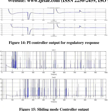
Figure 14: PI controller output for regulatory response

Figure 15: Sliding mode Controller output

[image:9.612.50.293.468.702.2]

From the figure 15 the performance of the controller was analysed. Here the controller gives the oscillating output, because sliding mode controller takes the current value of 4 tanks as feedback and gives the output with respect to change in feedback. To attain the set point Sliding mode controller switches trajectory between the sliding mode surfaces which results in oscillation in controller output.

TABLE 4

PERFORMANCE ANALYSIS

Minimum Phase Non-Minimum Phase

Open loop response

1. The operating region for tank 1 and 2 is 15 and 16cm respectively.

1. The operating region for tank 1 and 2 is 12.5 and 13cm respectively. With PI

controller

1. Settling time is nearly 300sec. 2. Peak over shoot is

about 2.7cm.

1. Settling time is nearly 800sec.

SMC and PI Regulatory Response

1. Peak over shoot for SMC is 0.5cm and for PI is 2.5cm. 2. Response time for

SMC is 20 sec and for PI is 50 sec.

1. Peak over shoot for SMC is 1cm and for PI is 4.5cm. 2.Response time for

SMC is 20 sec and for PI is more than 100 sec.

SMC and PI Servo Response

1. Peak over shoot is not present in SMC but for PI is 2.5cm. 2. Response time is 50

sec for SMC and 200 sec for PI.

1. Peak over shoot is 0.5cm for SMC and for PI is 4cm. 2. Response time is 50

sec for SMC and more than 800 sec for PI

IX. CONCLUSION

The Quadruple tank process has been discussed and it is very well suited for demonstrating minimum phase and non-minimum phase system. The effects of coupling and performance limitations in multivariable control system are investigated. The step responses of PI controller for both minimum and non-minimum phase have overshoot, oscillations and the settling time was very large.

Particularly in case of non-minimum phase, the PI controller failed to control the level of the tanks at desired set point. The multivariable transmission zero calculation shows that there will be a RHP zero present in non-minimum phase case. The RGA analysis also indicates that the non-minimum phase is difficult to control because the value of the split ration is less than zero ( ). Sliding mode control algorithm uses narrow zone of stability where the system has non-minimum phase behaviour. In spite of split fractions change and affected transmission zero locations; the control algorithm uses constant value of split fraction to keep the order of the controller model low. This uncertainty is found to be easily handled by the sliding mode controller.

REFERENCES

[1] K. H. Johansson. Relay feedback and multivariable control. PhD thesis, Department of Automatic Control, Lund Institute of Technology, Sweden, November 1997.

[2] K. H. Johansson. The Quadruple-Tank Process - A multivariable laboratory process with an adjustable zero. IEEE Transactions On Control Systems Technology, Vol. 8, No. 3, May 2000.

[3] S. M. Mahdi Alavi and Martin J. Hayes. Quantitative Feedback Design for a Benchmark Quadruple Tank Process. ISSC 2006, Dublin Institute of Technology, June 28-30.

[4] Qamar Saeed, Vali Uddin and Reza Katebi. Multivariable Predictive PID Control for Quadruple Tank. World Academy of Science, Engineering and Technology, 2010.

[5] Johansson KH, Horch A, Hansson A. Teaching multivariable control using the quadruple tank process. In: Proceeding of the 38th conference on decision & control; December 1999.

[6] K. Numsomran, T. Witheephanich, K. Trisuwannawat, and K. Tirasesth, I-P controller design for quadruple-tank system. Proc. 5th Asian Control Conference, 2004, Australia.

[7] Pinak Pani Biswas, Rishi Srivastava, Subhabrata Ray, Amar Nath Samanta. Sliding mode control of quadruple tank process. Science Direct, Mechatronics, 13 January 2009.