H e l m h ol t z b r i g h t s p a ti al s olit o n s
a n d s u rf a c e w a v e s a t p o w e r-l a w
o p ti c al in t e rf a c e s
C h ri s ti a n , JM, M c C oy, E, M c D o n a l d , GS, S a n c h e z-C u r t o , J a n d
C h a m o r r o-P o s a d a , P
h t t p :// dx. d oi.o r g / 1 0 . 1 1 5 5 / 2 0 1 2 / 1 3 7 9 6 7
T i t l e
H el m h ol tz b r i g h t s p a ti al s oli t o n s a n d s u r f a c e w a v e s a t
p o w e r-l a w o p ti c al i n t e rf a c e s
A u t h o r s
C h ri s ti a n , JM, M c C oy, E , M c D o n a l d , GS, S a n c h e z-C u r t o , J
a n d C h a m o r r o-P o s a d a , P
Typ e
Ar ticl e
U RL
T hi s v e r si o n is a v ail a bl e a t :
h t t p :// u sir. s alfo r d . a c . u k /i d/ e p ri n t/ 2 6 9 2 8 /
P u b l i s h e d D a t e
2 0 1 2
U S IR is a d i gi t al c oll e c ti o n of t h e r e s e a r c h o u t p u t of t h e U n iv e r si ty of S alfo r d .
W h e r e c o p y ri g h t p e r m i t s , f ull t e x t m a t e r i al h el d i n t h e r e p o si t o r y is m a d e
f r e ely a v ail a bl e o nli n e a n d c a n b e r e a d , d o w nl o a d e d a n d c o pi e d fo r n o
n-c o m m e r n-ci al p r iv a t e s t u d y o r r e s e a r n-c h p u r p o s e s . Pl e a s e n-c h e n-c k t h e m a n u s n-c ri p t
fo r a n y f u r t h e r c o p y ri g h t r e s t r i c ti o n s .
Volume 2012, Article ID 137967,21pages doi:10.1155/2012/137967
Research Article
Helmholtz Bright Spatial Solitons and Surface Waves at
Power-Law Optical Interfaces
J. M. Christian,
1, 2E. A. McCoy,
1G. S. McDonald,
1J. S´anchez-Curto,
2and P. Chamorro-Posada
21Joule Physics Laboratory, School of Computing, Science and Engineering, Materials & Physics Research Centre, University of Salford, Greater Manchester M5 4WT, UK
2Departamento de Teor´ıa de la Se˜nal y Comunicaciones e Ingenier´ıa Telem´atica, Universidad de Valladolid, ETSI Telecomunicaci´on, Campus Miguel Delibes Paseo Bel´en 15, E-47011 Valladolid, Spain
Correspondence should be addressed to J. M. Christian,[email protected]
Received 24 April 2012; Accepted 31 May 2012
Academic Editor: Alan Migdall
Copyright © 2012 J. M. Christian et al. This is an open access article distributed under the Creative Commons Attribution License, which permits unrestricted use, distribution, and reproduction in any medium, provided the original work is properly cited.
We consider arbitrary angle interactions between spatial solitons and the planar boundary between two optical materials with a single power-law nonlinear refractive index. Extensive analysis has uncovered a wide range of new qualitative phenomena in non-Kerr regimes. A universal Helmholtz-Snell law describing soliton refraction is derived using exact solutions to the governing equation as a nonlinear basis. New predictions are tested through exhaustive computations, which have uncovered substantially enhanced Goos-H¨anchen shifts at some non-Kerr interfaces. Helmholtz nonlinear surface waves are analyzed theoretically, and their stability properties are investigated numerically for the first time. Interactions between surface waves and obliquely incident solitons are also considered. Novel solution behaviours have been uncovered, which depend upon a complex interplay between incidence angle, medium mismatch parameters, and the power-law nonlinearity exponent.
1. Introduction
A light beam impinging on the interface between two dissimilar dielectric materials is a fundamental optical geometry [1–12]. After all, the single-interface configuration is an elemental structure that facilitates more sophisticated device designs and architectures for a diverse range of photonic applications. The seminal work of Aceves et al. [6,7] some two decades ago considered perhaps the simplest scenario, where a spatial soliton (i.e., a self-trapped and self-stabilizing optical beam) is incident on the boundary between two different Kerr-type materials. Their intuitive approach reduced the full complexity of the electromag-netic interface problem to something far more tractable, namely, the solution a scalar equation of the inhomogeneous nonlinear Schr¨odinger (NLS) type. The development of an equivalent-particle theory [3–6] provided an enormous level of insight into the behaviour of scalar solitons at material
wave optics must be applied with care since, in potentially off-axis regimes, it holds true only where angles (in the laboratory frame) of incidence, reflection, and refraction with respect to the reference direction are negligibly (or near-negligibly) small.
Recently, we proposed the first scalar model of spatial solitons at interfaces that is valid across the entire angular range [17, 18]. By respecting the essential role played by Helmholtz diffraction [19–24], the angular restriction was lifted while retaining an intuitive and manageable envelope equation. Preliminary analyses considered bright [17, 18] and dark [25,26] spatial solitons incident on the boundary between dissimilar Kerr-type materials. They focused on establishing and developing the propagation aspects of our Helmholtz interfaces approach. By enforcing appropriate continuity conditions at the interface, a Snell’s law for Kerr spatial solitons was derived whose validity was tested and confirmed by extensive numerical computations. Here, we take the first steps in a systematic study of the materials aspects of nonlinear beam-interface interactions. The sim-plest non-Kerr system one might consider is a class of host media whose refractive indexnNL(E) has a generic
power-law dependence on the (complex) electric field amplitudeE
[27–29]:
nNL(E)= α
2n0|E|
q,
(1)
whereαis a positive coefficient,n0is the linear index (at the
optical frequency), and the exponentqlies within the range 0< q <4. Typically, the nonlinear response of the medium is assumed to be weak so thatαEq0/n0O(1), whereE0is the
peak field amplitude.
Power-law models have played a key role in the theory of nonlinear waves for the past three decades [30,31]. Indeed, [32] provides an excellent review of the fundamental impor-tance of model (1) in photonics contexts. Materials that fall into this broad category include some semiconductors (e.g., InSb [33] and GaAs/GaAlAs [34]), doped filter glasses (e.g., CsSxSex−2 [35,36]), and liquid crystals [32]. One expects
non-Kerr regimes (whereqdeviates from the value of 2) to give rise to a diverse range of new quantitative and qualitative phenomena. The physical basis for this expectation lies in the idealized nature of the Kerr response. In a range of materials, one can often find higher-order nonlinear effects coming into play. Perhaps the most obvious example of the breakdown of Kerr-type behaviour is optical saturation, where the refractive index change becomes bleached in the presence of sufficiently high-intensity illumination. In such cases, model (1) with q < 1 can be used to describe generic leading-order corrections from a saturable (dispersive) nonlinearity [35,36].
In this paper, a detailed account is presented of arbitrary-angle refraction of spatial solitons at the interface between dissimilar power-law materials. Also of intrinsic interest are nonlinear surface waves (i.e., localized modes that travel along the boundary). This fundamental class of excitation has been the subject of previous power-law studies involving a single interface [35–39] and guided waves in multilayer
structures (e.g., slab waveguides) [40–43]. Stability char-acteristics have been inferred from inspection of power-propagation constant solution branches. However, to the best of our knowledge, direct verification of such predictions [37–43] (e.g., through numerical solution of the underlying nonlinear Helmholtz equation) has been absent from the literature to date. Rather, computational studies of surface waves tend to have been in the limit of slowly varying envelopes and nonlinear Schr¨odinger-type models, typically of the diffusive-Kerr [44, 45], thermal [46], or saturable [47] type. Here, we investigate the stability of exact ana-lytical Helmholtz surface waves through direct numerical calculations. As a fairly stringent test of solution robustness, we also report on some key findings concerning arbitrary-angle interactions between surface waves and solitons. In beam-refraction and surface-wave contexts, simulations have uncovered strikingly distinct behaviours as the exponent
q is varied and across a range of quasi-paraxial and fully nonparaxial angular regimes.
The layout of this paper is as follows. In Section 2, we propose a governing equation for scalar optical fields in two adjoining power-law materials with dissimilar medium coefficients. Exact analytical bright solitons are presented for both media, and these solutions are used as a nonlinear basis to derive a generalized Helmholtz-Snell law. In Section 3, extensive computations test predictions of the new refraction law over a range of system parameters. We also extend our first calculations of the Goos-H¨anchen (GH) shifts [48] in the Helmholtz angular regime [49] with power-law nonlinearities. Nonlinear surface waves are derived in
Section 4, and simulations provide what appears to be the first full investigation of the stability properties of this new class of Helmholtz solution. We conclude, inSection 5, with some comments about the impact of our results.
2. Helmholtz Model for Scalar
Soliton Refraction
The formalism of Helmholtz soliton theory [23,24] is now deployed to develop a framework for describing refraction phenomena in wider classes of nonlinear optical materials. This type of modelling approach is valid when the beam waistw0 is much broader than its free-space carrier
wave-lengthλ, such that ε ≡ λ/w0 O(1). Ultranarrow beam
corrections to the governing equation, typically obtained from single-parameter (i.e., ε-based) order-of-magnitude analyses of fully-nonlinear Maxwell equations [50–55], are unnecessary in such regimes.
2.1. Governing Equation. Within the scalar approximation [19–24], we consider an electric field of the form
known that the complex spatial field E(x,z) satisfies the Helmholtz equation
∂2E
∂z2 +
∂2E
∂x2 +
ω2
c2n 2
j(E)E=0, (3) where c is the vacuum speed of light. The refractive index distribution nj(E) on either side of the boundary is introduced through n2
j(E) ≡ n20j + αj|E|q, where n0j is the linear index at frequency ω and αj is a nonlinearity coefficient. To facilitate comparison with our earlier work [17, 18, 25, 26], we look for travelling-wave solutions to (3) of the formE(x,z) = E0u(x,z) exp(ik1z). Here,E0 is a
(real) scale factor determining electric-field units,u(x,z) is the dimensionless envelope, and exp(ik1z) biases the solution
in the forward longitudinal direction (taken to bez), where
k1 ≡ n01ω/c is the (linear) propagation constant of the
carrier wave in medium 1. It then follows that u satisfies the inhomogeneous equation
∂2u
∂z2 + i2k1
∂u ∂z+
∂2u
∂x2 +
ω2
c2α1E
q
0|u|qu
=
k2 1
1−n202
n2 01
+ω
2
c2α1E
q
0
1−α2
α1
|u|q
h(x,z)u, (4)
where h(x,z) is a Heaviside function that is equal to zero (unity) in the domain of medium 1 (medium 2). Equation (4) may be normalized with respect to the parameters in medium 1, in which case the following governing equation may be derived without further approximation [17,18,56,
57]:
κ∂
2u
∂ζ2 + i
∂u ∂ζ +
1 2
∂2u
∂ξ2 +|u|
qu=Δ
4κ+ (1−α)|u|
q h(ξ,ζ)u. (5)
The dimensionless longitudinal and transverse coordinates areζ = z/LD andξ = 21/2x/w0, respectively, whereLD =
k1w20/2 is the diffraction length of a reference (paraxial)
Gaussian beam. The inverse beam width is quantified by
κ=1/(k1w0)2=ε2/4π2n201O(1), whereε≡λ/w0, and the
field amplitude scales withE0=(2n201/α1k1LD)
1/q
. Model (5) is supplemented by the mismatch parameters [17,18,25,26]
Δ≡1−n
2 02
n2 01
, (6a)
α≡α2
α1
, (6b)
which determine how the linear and nonlinear refractive properties of the system change as one traverses the bound-ary.
Equation (5) allows one access to material scenarios where Δ < 0 (i.e., configurations with n02 > n01) [17,
18, 25, 26]. By contrast, the scalings deployed in classic paraxial theory [8,9] restrict those models to consideration of regimes withΔ >0. It is also apparent that settingκ≈0 in an attempt to recover the paraxial model is going to lead to complications when handling the linear mismatch term
Δ/4κ. The physical and mathematical difficulties of interpret-ing the paraxial approximation as the sinterpret-ingle-parameter limit
κ≈0 have been discussed at length elsewhere [23,24]; it is particularly well illustrated by interface geometries.
2.2. Solitons as a Nonlinear Basis. When investigating the re-fraction of nonlinear light beams at material boundaries, it is essential to have an appropriate set of basis functions with which to formulate the problem. Such a basis is provided by the underlying exact analytical Helmholtz solitons [56]. In the following analysis, we align the interface along thezaxis so that it is located at transverse positionx =0. Medium 1 (the domain of the incident beam, whereh=0) is taken to occupy the half-plane−∞ ≤ x < 0, while medium 2 (the domain of the refracted beam, whereh=+1), occupies 0≤
x≤+∞.
In medium 1, the governing equation (5) becomes
κ∂
2u
∂ζ2 + i
∂u ∂ζ +
1 2
∂2u
∂ξ2 +|u|
qu=0.
(7)
Sufficiently far from the interface, (7) admits exact analytical solitons of the form [56]
u(ξ,ζ)=η0sech2/q
⎛
⎝aξ−Vincζ
1 + 2κV2 inc ⎞ ⎠ ×exp ±i
1 + 4κβ0
1 + 2κVinc2
Vincξ+ ζ
2κ
×exp
−i ζ 2κ
,
(8a)
whereη0is the peak amplitude of the beam,a=q[ηq0/(2 +
q)]1/2determines the (inverse) solution width, and
β0=2 η
q
0
2 +q (8b)
quantifies nonlinear phase shift through the (typically small) quantity 4κβ0. The ± sign flags evolution in the
forward/backward longitudinal direction. The propagation angle of the beam in the laboratory (i.e., the (x,z)) frame, denoted by θinc and measured with respect to the z axis,
is related to the transverse velocity parameterVinc through
tanθinc=(2κ)1/2Vinc[23,24]. In medium 2,usatisfies
κ∂
2u
∂ζ2 + i
∂u ∂ζ +
1 2
∂2u
∂ξ2 −
Δ
4κu+α|u|
q
θref
θinc 0
(n01,α1)
z x
(n02,α2)
(a)
θref
0
θinc
(n01,α1)
z x
(n02,α2)
(b)
θref
0
θinc
(n01,α1)
z x
(n02,α2)
(c)
Figure 1: Schematic diagram illustrating (a) internal (θref < θinc) and (b) external (θref > θinc) refraction in the laboratory frame. The
transparency condition (θref =θinc) is shown in part (c). External refraction regimes tend to be highly angular and cannot be adequately described by the paraxial approximation.
and one may derive similar families of solitons,
u(ξ,ζ)=η0sech2/q
⎛
⎝a√αξ−Vrefζ
1 + 2κVref2
⎞ ⎠ ×exp ±i
1−Δ+ 4κβ0α
1 + 2κV2 ref
Vrefξ+ ζ
2κ
×exp
−iζ 2κ
.
(10)
Note that the connection between transverse velocity Vref
and propagation angleθref, that is, tanθref = (2κ)1/2Vref, is
unaffected by the (additional, linear) termΔ/4κin (9) or by the nonlinear coefficientα. The geometry of these solitons, and their inherent stability against perturbations to the local beam shape, was explored in detail in [56].
2.3. Phase Continuity and Refraction. In recent analyses, we have shown that arbitrary-angle refraction is well described by anticipating that the phase distribution of the light be continuous across the interface [17, 18,25,26]. Matching the phases of solutions (8a) and (10) atx = 0 leads to the requirement that
±
1 + 4κβ0
1 + 2κV2 inc
= ±
1−Δ+ 4κβ0α
1 + 2κV2 ref
. (11) Hence, continuity is possible if and only if the incident and refracted solitons share a common longitudinal sense (i.e., both must be in either the forward or backward directions). By rearranging (11), one can show thatVrefis related toVinc
through
V2
ref=Vinc2 −
1 2κ
1 + 2κVinc2
1 + 4κβ0
Δ+ 4κβ0(1−α)
. (12) Expressed in this way, (12) provides a helpful form “V2
ref =
V2
inc +deviation,” where the sign of the deviation can be
analysed separately. It is then instructive to define a net mismatch parameterδas [17,18]
δ≡Δ+ 4κβ0(1−α). (13)
This parameter can be interpreted as the sum of linear and nonlinear mismatches in material parameters. Its sign fully
characterizes beam refraction. When δ > 0, one has that
V2
ref < Vinc2 , which is equivalent toθref < θinc. This regime
is referred to as internal refraction, and it corresponds to the situation where the beam in medium 2 is deviated toward the interface (seeFigure 1(a)). Conversely,δ <0 implies that
Vref2 > Vinc2 or, equivalently,θref> θinc. This external refraction
regime corresponds to the beam in medium 2 being bent away from the interface (see Figure 1(b)). The special case of δ = 0 is the transparency condition, where linear and nonlinear index mismatches oppose each other exactly so that V2
ref = Vinc2 (or θref = θinc). The interface is thus
essentially transparent to the incident beam (seeFigure 1(c)), which experiences no net change in dielectric properties as it crosses the boundary. It is interesting to note that the absence of an interface provides a parameter subset (i.e.,Δ=0 and
α=1) that satisfies the transparency condition identically. 2.4. The Helmholtz-Snell Law for Spatial Solitons. By recog-nizing the rotational symmetry inherent to Helmholtz spatial solitons [23, 24, 56], it becomes clear that “forward” and “backward” designations are arbitrary. The only physical distinction between the two families is the propagation direction relative to the observer. By deploying trigonometric identities to eliminate velocities Vinc andVref, the forward
and backward solutions in each medium may be written as
u(ξ,ζ)=η0sech2/q
a
ξcosθinc−√ζ
2κsinθinc
×exp
⎡ ⎣i
1 + 4κβ0
2κ
ξsinθinc+√ζ
2κcosθinc
⎤ ⎦
×exp
−i ζ 2κ
,
(14a)
and
u(ξ,ζ)=η0sech2/q
a√α
ξcosθref−√ζ
2κsinθref
×exp
⎡ ⎣i
1−Δ+ 4κβ0α
×
ξsinθref+√ζ
2κcosθref
×exp
−i ζ 2κ
.
(14b)
In this representation, the angles are bounded by
−180◦ < θinc, ref ≤ +180◦ with respect to the z-axis.
By matching the solution phase at ξ = 0, one can obtain a compact Helmholtz-Snell refraction law involving laboratory-frame angles:
γn01cosθinc=n02cosθref, (15a)
where
γ≡
1 + 4κβ0
1 + 4κβ0α(1−Δ)−1
1/2
. (15b)
It is worthwhile noting that (15a) has a form which is almost exactly identical to that encountered when studying the classic electromagnetic problem of plane wave refraction at the boundary between different linear dielectrics. Thus, the single correction factorγcaptures the interplay between finite-waist beams (through the appearance of κ) and discontinuities in both the linear and nonlinear properties of the adjoining media. The exponentq appears implicitly throughβ0.
When a beam encounters the boundary with a rarer medium, there is little penetration of light across that boundary until the incidence angle exceeds a critical value, denoted byθcrit. At criticality, whereθinc=θcrit, the trajectory
of the incident beam is deviated so that, in principle, the outgoing beam travels along the interface (i.e., θref = 0).
Applying this condition to law (15a) and (15b) leads to an analytical prediction for θcrit in terms of the mismatch
parametersΔandαand also the solution parameter 4κβ0:
tanθcrit=
Δ+ 4κβ0(1−α)
1−Δ+ 4κβ0α
1/2
. (16) In practice, one rarely finds the refracted soliton travelling along the interface boundary since other effects tend to appear (we will return to this point later).
2.5. Universal versus Specific Representations. There is clearly a universal flavour about (12), (13), (15a), (15b) and (16). For instance, there is no explicit mention of the system nonlinearity so that refraction is fully described by the mismatch parameters Δ and α and the beam parameter 4κβ0. These equations are, in fact, more general than they
first appear; for instance, laws of exactly the same structure govern the refraction of plane waves in power-law materials: a wave with real amplitudeu0hasβ0≡uq0(it is noteworthy
that the refraction analysis for plane waves does not capture the modulational instability of such solutions in the single power-law context [58]).
The power-law nature of the problem becomes apparent after one substitutes forβ0from (8b). Theγfactor (c.f. (15b))
then becomes
γ=
1 + 8κηq0
2 +q−1
1 + 8κηq0α
2 +q−1(1−Δ)−1 1/2
, (17a)
while the relation for the critical angle (c.f. (16)) is given by
tanθcrit=
Δ+ 8κη0q
2 +q−1(1−α) 1−Δ+ 8κηq0α
2 +q−1
1/2
, (17b)
and the net mismatch parameter (c.f. (13)) is δ = Δ+ 8κηq0(1−α)/(2 +q).
3. Simulations of Solitons at
Power-Law Interfaces
The Helmholtz type of off-axis nonparaxiality demands that the inequalities κ O(1) and 4κβ0 O(1) are always
met, which is equivalent to the simultaneous requirements of broad beams with moderate intensities, respectively [23,
24,56]. Here, attention is restricted to configurations where the mismatch parameters are relatively small, typicallyα =
O(1) and |Δ| O(1). We now proceed with a three-stage analysis. The simplest case to consider first is that of linear interfaces. We then move on to investigate nonlinear interfaces and conclude by noting the dependence of GH shifts [48,49] on the nonlinearity exponentq. Stable solitons of the homogeneous power-law Helmholtz model tend to exist in the continuous interval 0 < q < 4 [27,56]. For definiteness, we consider here only three discrete values:q=
1 (sub-Kerr), 2 (Kerr), and 3 (super-Kerr).
3.1. Solitons at Linear Interfaces. From (13), linear interfaces are defined by the inequality 4κβ0|1−α| |Δ|. To isolate
the effects of a linear-index change alone, we set α = 1.0 so that δ = Δ. One therefore finds the existence of a critical angle in regimes where Δ > 0 (since n02 < n01).
The following simulations consider q = 1.Figure 2shows generally good agreement between theoretical predictions and full numerical calculations whenκ=2.5×10⁻³; the level
of agreement is improved even further whenκ=1.0×10⁻⁴.
The fact that smaller values ofκgive rise to better theory-numerics agreement, despite the increased magnitude of the linear-interface perturbation term atΔ/4κ, invites comment. We suspect that one possible explanation may lie in the origin of the Helmholtz-Snell law, whereby one matches solution phase (but not amplitude) at the boundary: the matching condition thus takes no account of amplitude curvature. In the laboratory frame, broader beams (i.e., those characterized by smallerκvalues) tend to have lower amplitude curvature, and the corresponding spatial solitons (which play the role of nonlinear basis functions) thus map much more consistently onto the inherent assumptions of the analytical approach.
0 2 4 6 8 10
0 2 4 6 8 10
θinc(degrees)
θref
(deg
re
es)
(a)
0 2 4 6 8 10
0 2 4 6 8 10
θinc(degrees)
θref
(deg
re
es)
|Δ| =0.001
|Δ| =0.0025
|Δ| =0.005
|Δ| =0.01
(b)
Figure 2: Comparison of the theoretical Snell’s law given by (15a)
and (15b) (lines) against full numerical computations (points) for a unit-amplitude (η0=1.0) spatial soliton at a linear interface (α=
1.0) withq=1 and when (a)κ=2.5×10⁻³and (b)κ=1.0×10⁻⁴.
Curves below (above) theθref=θincline haveΔ >0 (Δ <0), so that the refraction is internal (external).
reminiscent of those reported in previous studies [56], and be accompanied by a radiation pattern. Computations [59] have verified the effective independence of the refraction angleθref
with respect to the incident amplitudeη0. Accordingly, the
curves in Figure 2 are essentially insensitive to q; they are quantitatively very similar to those obtained forq =2 [10]
and (whenθincis sufficiently aboveθcritin internal-refraction
regimes) forq=3.
Any interaction between a spatial soliton and an interface generally involves three distinct components: a reflected beam, a refracted beam (sometimes more than one), and radiation. The way in which the incident energy is distributed amongst these components depends on a complicated interplay between the interface and beam parameters, and also the incidence angle. At very small angles (e.g., θinc <
1◦), the interaction can be highly inelastic and nonadiabatic (especially in external refraction regimes). Crucially, the single refracted soliton (as predicted inSection 2) dominates as θinc approaches even modest nonparaxial angles, with
reflected and radiation components hardly excited at all. The Helmholtz-Snell law embodied by (15a) and (15b) is, of course, most valid in such regimes.
3.2. Solitons at Nonlinear Interfaces. Nonlinear interface effects dominate beam refraction when 4κβ0|1 − α|
|Δ|. Without loss of generality, we isolate such effects by settingΔ = 0 so that the net mismatch parameter is given by δ = 4κβ0(1−α) = 8κη0q(1−α)/(2 + q). Refraction
thus becomes far more sensitive toκ in nonlinear regimes (compare this to linear regimes, whereδ=Δis independent ofκ). Theoretical predictions are shown inFigure 3. While there is generally good agreement with numerics for both
κ = 2.5×10⁻³ andκ = 1.0×10⁻⁴ when α ≈ 1.0, the fit becomes less reliable forα = 2.0 and α =0.3. For such parameters, the nonlinear refractive index change across the boundary is no longer small: one cannot expect to find such a close match because of strong nonlinear effects (e.g., beam splitting and radiation phenomena). While the fit is clearly better for broader beams (κ =1.0×10⁻⁴), the Helmholtz-Snell predictions for narrower beams (κ = 2.5×10⁻³) are still in good qualitative agreement.
Detailed attention is first paid to regimes with α > 1 (external refraction, since δ < 0), where the nonlinearity is stronger in the second medium. Since the width of the refracted soliton is proportional toα−1/2, it follows that the
beam must become narrower as it crosses the interface. In this type of material regime, the incident soliton always has sufficient energy flow to excite a self-trapped soliton-like state in medium 2.
Simulations have shown that nonlinear external refrac-tion tends to induce stronger oscillarefrac-tions in the parameters (amplitude, width, and area = amplitude ×width) of the outgoing beam than in the linear case. Such oscillations are not captured by the adiabatic analysis in Section 2
(which anticipates a stationary state), but one expects their appearance intuitively. Qualitatively different effects can appear at quasi-paraxial incidence angles as the exponent
q is varied; an illustrative example is shown in Figure 4
for θinc = 3◦ when α = 2.0. A unit-amplitude soliton
0 2 4 6 8
0 2 4 6 8
θinc(degrees)
θref
(deg
re
es)
(a)
0 0.5 1 1.5 2 2.5
0 0.5 1.5 2.5
θinc(degrees)
θref
(deg
re
es)
1 2
α=0.9
α=0.7
α=0.5
α=0.3
α=1.1
α=1.3
α=1.5
α=2
(b)
Figure 3: Comparison of the theoretical Snell’s law given by (15a)
and (15b) (lines) against full numerical computations (points) for a unit-amplitude (η0 = 1.0) spatial soliton at a nonlinear interface (Δ = 0) withq = 1 and when (a) κ = 2.5×10⁻³ and (b) κ=1.0×10⁻⁴. Curves below (above) theθref=θincline are labelled
by the right-hand (left-hand) legend and haveα < 1 (α > 1) so that refraction is internal (external). Note that the numerical datapoints forα=0.3 andα=0.5 are very close together in both panes.
component in the form of radiation modes). Since the internally refracted beam carries away some of the momen-tum of the incident beam, it follows that the dominant refracted beam travels at a smaller angle than that predicted by (15a) and (15b). This type of splitting is not present for unit-amplitude solitons with q = 2 (see Figure 4(b)), though it may appear for incident solitons with higher peak intensities [60]. In such cases, the properties of the daughter solitons may be quantified with recourse to inverse scattering techniques. Splitting is also absent atq=3 (seeFigure 4(c)), though one finds quite a complicated radiation ripple pattern in the second medium.
Refraction in nonparaxial regimes tends to be a much cleaner process, with little radiation generated by the beam-interface interaction in comparison with quasi-paraxial regimes. Even at modest angles (e.g.,θinc =30◦), where the
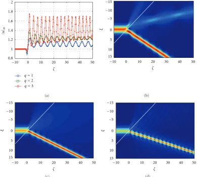
interface perturbation is distributed over a relatively short interaction length, the quantitative characteristics of the outgoing beam depend crucially on the power-law exponent. Both the depth of modulation and (longitudinal spatial) frequency of the oscillations tend to increase with q, as shown inFigure 5(a). Whenq=2, the oscillations tend to vanish in
ζ; forq = 1 and 3, they survive in the long-term evolution (this is also true for the oscillations shown inFigure 4(a)). A more detailed comparison of how the q affects beam refraction is presented in Figures5(b)–5(d).
For material combinations withα < 1 (internal refrac-tion, since δ > 0), the nonlinearity is weaker in the second medium. In that case, one should expect a critical angle to exist (in accordance with (17b)). If the incident soliton survives the interaction with the interface, then the refracted beam may be expected to undergo self-reshaping oscillations in its parameters, with the overall trend being toward an increase in solution width. Simulations have confirmed this to be the case, with diffractive broadening generally accompanied by a reduction in peak amplitude (seeFigure 6(a))—these oscillations are reminiscent of those uncovered previously for perturbed initial-value problems [56].
Computations have uncovered a range of q-dependent effects, an illustrative sample of which is shown inFigure 6
for beams with κ = 2.5 ×10⁻³, a nonparaxial incidence angleθinc=30◦, and a nonlinear mismatch ofα=0.5. The
(longitudinal spatial) frequency of the reshaping oscillations tends to decrease with increasing q (c.f., the increase with
q whenα > 1). Also at higher q values (e.g., forq = 3), a threshold phenomenon can appear whereby the energy-flow [56] of the incident soliton may not be great enough to excite a refracted beam (if the energy flows associated with solutions (8a) and (10) are denoted byWinc andWref,
respectively, then it can be shown that Wref ≈ Winc/α1/2).
This instability is shown inFigure 6(d): upon colliding with the interface, the beam breaks up into radiation (this scenario is also present at quasi-paraxial incidence angles above the critical angleθcrit).
|
u
|m
−10 0 10 20 30 40 50
0.8 1 1.2 1.4 1.6 1.8 2
ζ
q=1
q=2
q=3
(a)
−10 0 10 20 30 40 50
15 10 5 0
−5
−10
−15
ζ
ξ
(b)
−10 0 10 20 30 40 50
15 10 5 0
−5
−10
−15
ζ
ξ
(c)
−10 0 10 20 30 40 50
15 10 5 0
−5
−10
−15
ζ
ξ
[image:9.600.105.496.74.426.2](d)
Figure 4: External refraction of a unit-amplitude (η0 = 1.0) spatial soliton at a nonlinear interface withα = 2.0 and a quasi-paraxial
incidence angleθinc=3◦whenκ=2.5×10⁻³. (a) Evolution inζof the peak amplitude|u|
mof the beam. (b), (c), and (d) show the full numerical solution|u(ξ,ζ)|of (5) when the nonlinearity exponent isq=1, 2, and 3, respectively.
angle must depend onq(a prediction supported by simple inspection of Figures 4, 5, and 6). At this point, it also becomes instructive to consider the trajectory of refracted beams more carefully. Detailed numerical calculations reveal that at quasi-paraxial incidence angles, the beam in the second medium tends to follow a straightline path. Such a simple notion of refraction, founded upon intuition from plane wave theory, is illustrated inFigure 7(a)for a nonlinear interface with α = 2.0 and a beam with θinc = 3◦
and κ = 2.5 ×10⁻³. However, if the incidence angle is increased into the nonparaxial domain (e.g.,θinc = 30◦), a
qualitatively different picture emerges. Now, the straightline path ξ −Vrefζ = 0 predicted by solution (10) defines an
average trajectory about which the refracted beam “snakes.”
Figure 7(b) quantifies this snaking effect for the external refraction simulations shown in Figures5(b)–5(d). Snaking is more apparent with sub-Kerr nonlinearities (i.e., where
q < 2), and it increases for narrower beams (i.e., larger values of κ) at a fixed amplitude (see Figure 8(a), where
η0=1.0). Beams with larger amplitudes also exhibit snaking,
but oscillations tend to be more rapid in the longitudinal direction (seeFigure 8(b)).
The snaking phenomenon is most pronounced in regimes withα >1, where the nonlinearity is stronger in the second medium. There is also an intrinsic dependence onθinc
that can be seen inFigure 7. For small angles of incidence, the incoming soliton experiences an interface perturbation that is distributed over a relatively long distance. The refracting beam is able to accommodate the inhomogeneity in the system since changes in focusing properties of the host medium occur gradually in the longitudinal direction. For larger-incidence angles, the effective beam-interface interaction length may be much shorter. Solitons impinging on the boundary then exhibit a sharp (rather than a gradual) perturbation whose action is to induce sustained oscillations.
0 5 10 15 20 0.8
1 1.2 1.4 1.6 1.8 2
ζ
−5
q=1
q=2
q=3
|
u
|m
(a)
−5 0 5 10 15 20
10 5 0
−10
−5
ζ
ξ
(b)
−5 0 5 10 15 20
10 5 0
−10
−5
ζ
ξ
(c)
−5 0 5 10 15 20
10 5 0
−10
−5
ζ
ξ
(d)
Figure 5: External refraction of a unit-amplitude (η0=1.0) spatial soliton at a nonlinear interface withα=2.0 and a nonparaxial incidence
angleθinc=30◦whenκ=2.5×10⁻³. (a) Evolution inζof the peak amplitude|u|
mof the beam. (b), (c), and (d) show the full numerical solution|u(ξ,ζ)|of (5) when the nonlinearity exponent isq=1, 2, and 3, respectively.
of a reflected beam relative to its position as predicted by geometrical optics. Extensive numerical investigations considered the interplay between incidence angleθinc,
mate-rial mismatches (Δ,α), and the nonparaxial parameter κ. Radiation-induced trapping was found to play a key role in determining the magnitude of the shift. Also uncovered were giant external GH shifts (in regimes with δ > 0 but where the second medium has a weaker nonlinearity (i.e.,
α < 1)). While a similar investigation of GH shifts in the power-law context is certainly outside our current scope, a small selection of results will now be presented to illustrate how they depend upon the nonlinearity exponent q.
We begin by considering linear interfaces and unit-amplitude incident solitons withκ =2.5×10⁻³. According
to (16), interfaces withΔ=0.0025 have a theoretical critical angle ofθcrit≈2.86◦(this value depends only very weakly on
q).Figure 9(a)gives a representative set of results. Inspection shows that, for anyθinc, the magnitude of the shift is generally
greater for systems with q = 1 than forq = 2 orq = 3. The true critical angle (which can only be found through full simulations) is also slightly greater than that predicted by theory (forq = 1 andq = 2,θcrit ≈ 3.016◦ andθcrit ≈
3.030◦; both angles exceed their theoretical values ofθcrit ≈
2.857◦andθcrit≈2.859◦, respectively). While the qualitative
behaviour of systems withq = 1 andq = 2 is largely very similar, strong qualitative differences have been uncovered in the case ofq =3. Asθincapproaches the theoretical critical
angle, the incident soliton often becomes unstable against the interface perturbation. Large amounts of radiation tend to be generated by the interaction (c.f.Figure 9(d)), so that there is essentially no reflected or refracted beam and a GH shift is thus not easily quantifiable (or even meaningful). However, whenθincis sufficiently aboveθcrit, the refraction angle is still
well described by theory.
GH shifts at nonlinear interfaces have also been analyzed; results are presented in Figure 10 forα = 0.7 and where system nonlinearity has been augmented by considering incident solitons with η0 = 2.0. Regimes with Δ =
0 25 50 75 100 125 0
0.2 0.4 0.6 0.8 1 1.2
ζ
q=1
q=2
q=3
|
u
|m
(a)
0 25 50 75 100 125
20 10 0
−10
−20
ζ
ξ
(b)
0 25 50 75 100 125
20 10 0
−10
−20
ζ
ξ
(c)
0 25 50 75 100 125
20 10 0
−10
−20
ζ
ξ
[image:11.600.103.498.73.431.2](d)
Figure 6: Internal refraction of a unit-amplitude (η0=1.0) spatial soliton at a nonlinear interface withα=0.5 and a nonparaxial incidence
angleθinc=30◦whenκ=2.5×10⁻³. (a) Evolution inζof the peak amplitude|u|
mof the beam. (b), (c), and (d) show the full numerical solution|u(ξ,ζ)|of (5) when the nonlinearity exponent isq=1, 2, and 3, respectively.
the true critical angle slightly exceeds theory). However, it is worth noting that the qualitative behaviour predicted by (16), namely that θcrit increases with q, is supported
by numerics. Close to the (true) critical angle, simulations show that there is a strong divergence in the GH shift (which becomes highly sensitive to θinc). Two other
gen-eral trends are that (i) GH shifts are larger (sometimes notably) for q = 1 than for q = 3; (ii) in nonlinear regimes, the GH shifts depend more strongly on q than for the case of linear interfaces (compare Figure 10 to
Figure 9(a)).
Figure 10(b)reveals new types of behaviour at power-law interfaces when q /=2. In particular, for q = 3 one enters a regime wherein the GH shift no longer increases monotonically withθinc; instead, there is a marked decrease
in the shift before the divergence at θinc ≈ θcrit sets in.
These results provide clear evidence that one can, quite reasonably, expect to find new qualitative phenomena in material regimes that deviate from the idealized Kerr-type response.
4. Helmholtz Nonlinear Surface Waves
Surface waves are well known in nonlinear photonics, being stationary localized light states that travel along the interface between different media. The transverse mode profiles are typically asymmetric due to the differences in dielectric properties defining the interface. We now derive the surface modes of model (5) using solitons (8a) and (10) as a nonlinear basis. These new solu-tions are most conveniently parameterized by β, which is related to the propagation constant in paraxial theory [27,
56].
4.1. Exact Analytical Solutions. To proceed, one seeks solu-tions to (5) of the form u(ξ,ζ) = F(ξ −ξj) exp(ikζζ) exp(−iζ/2κ), wherekζis the propagation constant andF(ξ−
ξj) is the (real) envelope profile that is centred onξj. After substituting for u and definingκk2
−10 0 10 20 30 40 0
10
15
20
ζ
−5
5
ξ0
(a)
0 4 8 12 16
0.4
0.8
1.2
ζ
20 0
ξ0
q=1
q=2
q=3
(b)
Figure 7: External refraction of a unit-amplitude (η0 = 1.0)
spatial soliton at a nonlinear interface with α = 2.0 when the incidence angle is (a) quasi-paraxial (θinc=3◦) and (b) nonparaxial (θinc = 30◦) for κ = 2.5×10⁻³. In (a), the trajectory of the
beam in the second medium is essentially a straight line. In (b), the trajectory oscillates (“snakes”) around the straight-line path predicted by the analysis in Section 2. Calculations of the beam centreξ0 were obtained by fitting the numerical solution at each longitudinal position to a trial function of the form ufit(ξ) =
η(ζ)sech2/q{a(ζ)[ξ−ξ0(ζ)]}. Black dashed lines: best-fit trajectory.
u(ξ,ζ)=
2 +q
2 β
1/q sech2/q
q
√
2β
1/2(ξ−ξ
1)
×exp
±i
1 + 4κβζ
2κ
exp
−i ζ 2κ
,
(18a)
while in medium 2
ξ0
0 4 8 12 16 20
−0.25
0
0.25
0.5
0.75
1
1.25
1.5
ζ
(a)
0 4 8 12 16 20
−0.25
0
0.25
0.5
0.75
1
1.25
1.5
ζ
κ=1×10⁻⁴
κ=1×10⁻³ κ=
2.5×10⁻³
κ=5×10⁻³
ξ0
(b)
Figure 8: External refraction of spatial solitons at a nonlinear
interface withα=2.0 for a nonparaxial angleθinc=30◦forq=1 and different values ofκ. The peak amplitude of the incident beam in each case is (a)η0=1.0 and (b)η0=2.0.
u(ξ,ζ)=
2 +
q
2 β
1
α
1 + Δ
4κβ
1/q
×sech2/q ⎡ ⎣√q
2β
1/2
1 + Δ
4κβ
1/2
(ξ−ξ2)
⎤ ⎦
×exp
±i
1 + 4κβ2ζ κ
exp
−iζ 2κ
.
(18b)
For a nonlinearity exponentq, the surface waves associated with any given interface are parameterized solely by β. The displacements ξ1 andξ2, as yet undetermined, can be
0 1 2 3
−40
0 40 80 120
θinc(degrees)
0.4 1 1.6 2.2
−10
0 10
q=1
q=2
q=3
Goos-H
¨anc
hen shift
(a)
−30 0 30 60 90 120 150
40 20 0
−20
−40
ζ
ξ
(b)
−30 0 30 60 90 120 150
40 20 0
−20
−40
ζ
ξ
(c)
−30 0 30 60 90 120 150
40 20 0
−20
−40
ζ
ξ
(d)
Figure 9: Demonstration of the GH shift for a unit-amplitude (η0 =1.0) spatial soliton at a linear interface withΔ=0.0025 and when
κ=2.5×10⁻³. (a) Variation of the GH shift with changing nonlinearity exponent q (theq=3 results (inset) closely follow those forq=2
until radiation effects come into play more strongly). (b), (c), and (d) show the full numerical solution|u(ξ,ζ)|of (5) whenq=1, 2 and 3, respectively (note that, over longer propagation lengths, the solution in (d) breaks up into radiation). The incidence angle in (b), (c), and (d) isθinc=3.016◦, which exceeds the (almostq-independent) critical angleθcrit≈2.86◦.
∂u/∂ξ or, equivalently, dF/dξ) across the interface. These conditions lead to
sech2/q
q
√
2β
1/2ξ
1
=
1
α
1 + Δ
4κβ
1/q
×sech2/q ⎡ ⎣√q
2β
1/2
1 + Δ
4κβ
1/2
ξ2
⎤ ⎦,
(19a)
tanh
q
√
2β
1/2ξ
1
=
1 + Δ
4κβ
1/2
×tanh
⎡ ⎣√q
2β
1/2
1 + Δ
4κβ
1/2
ξ2
⎤ ⎦,
(19b)
respectively. After some algebraic manipulation of (19a) and (19b), one finds that
ξ1=
√
2
q β
−1/2ln
1±√1−δ2
δ
(20a)
ξ2=
√
2
q β
−1/2
1 + Δ
4κβ
−1/2
ln ⎛ ⎝1±
1−μ2
μ
⎞
⎠, (20b)
where the parametersδandμare given byδ ≡[Δ/4κβ(α−
1)]1/2andμ≡[(Δ/4κβ)(1 +Δ/4κβ)−1
(1−1/α)−1]1/2.
4.2. Surface Wave Existence Criterion. For displacementsξ1
and ξ2 to be real, it must be that 0 < δ2 < 1 and 0 <
0 1 2 3
−15
0 15 30 45 60 75
θinc(degrees)
Goos-H
¨anc
hen shift
(a)
0 1 2 3
−15
0 15 30 45 60 75
θinc(degrees)
Goos-H
¨anc
hen shift 2.1 2.3 2.5
−20
−10
0 10
q=1
q=2
q=3
(b)
Figure 10: Numerical calculation of the GH shift for incident
spatial solitons withη0=2.0 at a nonlinear interface withα=0.7, (a)Δ= −0.001, and (b)Δ= −0.0025 whenκ=2.5×10⁻³(inset shows the behaviour of the shift forq=3 around the minimum).
inequality placed on the product 4κβ, namely, 4κβ >4κβmin,
where
4κβmin= Δ
α−1 (21) (it is interesting to note that 4κβmin is independent of
q). Thus, existence criterion (21) for Helmholtz surface
−6 −4 −2 0 2 4
0 1 2 3 4 5
ξ
6
q=1 (−)
q=1 (+)
q=3 (−)
q=3 (+)
|
u
(
ξ
, 0
)
|
(a)
−6 −4 −2 0 2 4
0 1 2 3 4 5
ξ
6
q=1 (+) q=3 (+)
q=1 (−) q=3 (−)
|
u
(
ξ
, 0
)
|
(b)
Figure 11: Nonlinear surface wave profiles forκ=2.5×10⁻³in (a)
regime 1 (withΔ=0.005 andα=2.0) and (b) regime 2 (withΔ= −0.005 andα=0.5). From (21), one has that 4κβmin=0.005 and henceβmin=0.5 for the solutions in (a), while 4κβmin=0.01 and henceβmin=1.0 in (b). In these profiles,β=2.0 so thatβ > βmin
in each case. The + and−signs in the legends refer to the choice of sign solution in (20a) and (20b).
waves explicitly involves the (inverse) beam size through the appearance ofκ. Since 4κβmust remain positive, it follows that surface modes are supported in two distinct parameter regimes: (i) regime 1:Δ > 0 andα >1 (i.e.,n202 < n201 and
α2 > α1) and (ii) regime 2:Δ < 0 and 0 < α < 1, (i.e.,
n02 > n01,α2 < α1). We mention, in passing, that (21) is
0 0.5 1 1.5 2 2.5 0
2 4 6 8
β
P
(
β
)
q=1 (−)
q=1 (+)
q=3 (−)
q=3 (+)
(a)
0 0.5 1 1.5 2 2.5
β 0
4 8 12 16
P
(
β
)
q=1 (+) q=3 (+)
q=1 (−) q=3 (−)
[image:15.600.54.287.70.508.2](b)
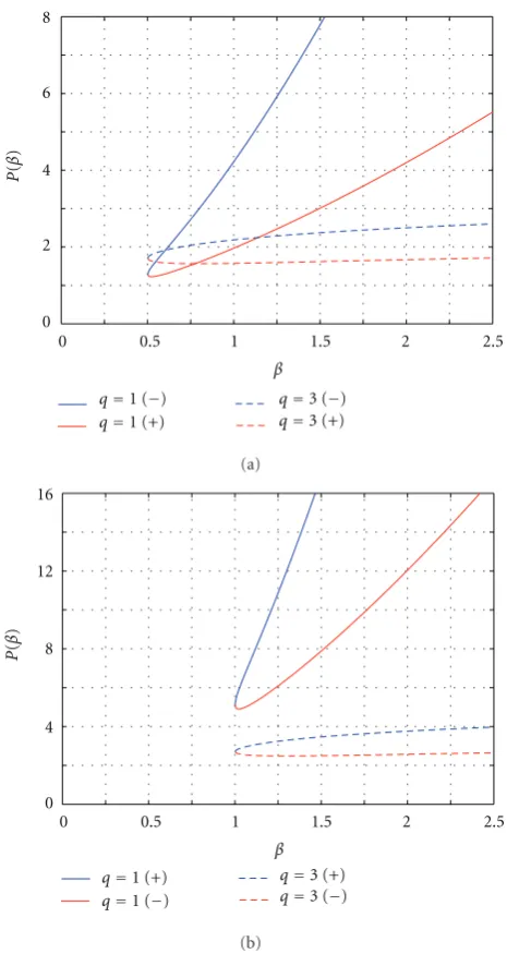
Figure 12: Power curves as a function of the propagation constant β, obtained from (22) withκ = 2.5×10⁻³. (a) Regime 1 with
Δ =0.005 andα = 2.0 and (b) regime 2 withΔ= −0.005 and
α = 0.5. The + and −signs in the legends refer to the choice of solution in (20a) and (20b). Lower (upper) solution branches appear as red (blue) lines, and each branch generally satisfies the VK stability criterion [61].
4.3. Solution Families and Wave Power. For both forward-and backward-propagating surface waves, there exist two solution families. The origin of this duality lies in solving simultaneous equations (19a) and (19b), where one is eventually obliged to find the roots of quadratic equations.
Figure 11reveals that, for fixed (Δ,α,β), the profile depends strongly on the nonlinearity exponent q. That is, the peak amplitude, width, and area all decrease with increasing
q. The difference between the two peak amplitudes and the distance of each solution peak from the interface also decrease with increasing nonlinearity exponent.
Since the surface wave profiles differ, it is plausible that the two families will not share the same stability properties. We begin an analysis of Helmholtz solutions (18a) and (18b) by considering the power P, where
Pβ;q≡
+∞
−∞dξ
u(ξ,ζ)2
, (22)
as a function of the free parameter β for different values of the nonlinearity exponent q. The energy-flow invariant
W [56] is related toP throughW(β)= ±(1 + 4κβ)1/2P(β), where the±sign here corresponds to forward- or backward-propagating envelopes (being distinct from the sign choice in (20a) and (20b)). A representative set of curves is shown inFigure 12, where it can be seen thatP(β) comprises two branches. In regime 1 (whereΔ >0 and α > 1), the lower (upper) branch corresponds to the−(+) sign in (20a) and (20b). This situation is reversed for regime 2 (whereΔ < 0, 0< α <1), in which the lower (upper) branch corresponds to the +(−) sign (see Figure 11). We note that for lower-branch solutions, the peak of the surface wave always resides in whichever medium has the lower linear refractive index.
Global trends in the parameter dependence of the modes profiles can be readily identified and discussed in the context of the two solution branches. For instance, one might fix Δ, β, and κ and consider the effect of varying α. In regime 1, one finds that upon increasing α, the upper-branch solutions tend to retain their shape while the lower-branch solutions experience a decrease in amplitude, width, and area. The separation between the pair of solutions also becomes greater, with each localized wave moving away from the interface. Asαis increased in regime 2, the lower-branch solutions tend to retain their shape while the upper-branch solution exhibits decreases in amplitude, width, and area. Also, the separation between the solutions tends to decrease with increasing α (so that the solutions move toward the boundary).
4.4. Surface Wave Stability. Except near the intersection point (whereβ≈βmin), bothP(β) branches satisfy the classic
Vakhitov-Kolokolov (VK) criterion for stability; namely,
dP/dβ > 0 [61]. Extensive simulations have revealed that lower-branch solutions always tend to remain self-trapped within the vicinity of the interface (so long as dP/dβ >
0) evolving with a stationary profile over arbitrarily long distances.
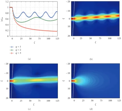
Upper-branch solutions tend to display a spontaneous instability in finite ζ. A set of typical results is shown in Figure 13 for regime 1 with Δ = 0.005 and α =
0 7 14 21 28 35 1.5
2 2.5 3 3.5 4
ζ
q=1
q=2
q=3
|
u
|m
(a)
0 7 14 21 28 35
10 5 0
−5
−10
ζ
ξ
(b)
0 7 14 21 28 35
10 5 0
−5
−10
ζ
ξ
(c)
0 7 14 21 28 35
10 5 0
−5
−10
ζ
ξ
(d)
Figure 13: Spontaneous instability of nonlinear surface waves lying on the upper solution branch ofFigure 12(a), whereκ=2.5×10⁻³and
β=2.0 (interface mismatch parameters areΔ=0.005 andα=2.0). (a) Evolution inζof the peak amplitude|u|mof the beam. (b), (c), and (d) show the full numerical solution|u(ξ,ζ)|of (5) when the nonlinearity exponent isq=1, 2, and 3, respectively. Note that the profiles of the input waves in (b) and (d) correspond to the upper-branch solutions shown inFigure 11(a).
(reshaping) daughter beam relative to the interface is largely insensitive toq.
Qualitatively different effects appear in regime 2 with
Δ= −0.005 andα=0.5; this time, the input wave is localized predominantly in medium 2 (compare with Figure 11(b)). After a finite propagation length, the surface wave bends smoothly away from the interface and is deflected deeper into medium 2. There is relatively little radiation shed in this process, and the localized wave suffers only a very small change to its shape (largely because the beam remains always on the same side of the interface, so does not encounter changes in refractive index). In common with regime 1, the instability growth rate increases withq.
4.5. Interactions between Solitons and Surface Waves. The stability of lower-branch surface waves is now investigated by considering their resilience against interactions with spatial
solitons. Only a brief summary is presented here since the primary motivation is to uncover qualitatively new effects that depend upon the exponent q (detailed quantitative analyses are reserved for future works). For definiteness, we present simulation results for collisions between a unit-amplitude (η0 = 1.0) soliton and surface waves in regimes
1 (Δ= 0.005,α =2.0) and 2 (Δ= −0.005,α = 0.5) with
β=2.0 andκ=2.5×10⁻³.
Regime 1 is considered first for a quasi-paraxial incidence angle ofθinc = 3◦ (see Figure 14). When q = 1, the two
distinct beams persist after the interaction. The path of the outgoing soliton has been deflected relative to its ingoing trajectory. The surface wave, on the other hand, survives as a localized spatial structure but can no longer be interpreted as a “surface wave” per se since it travels obliquely to (not along) the interface. This picture is qualitatively different for
0 10 20 30 40 50 60 1
1.4 1.8 2.2 2.6 3
ζ
q=1
q=2
q=3
|
u
|m
(a)
0 10 20 30 40 50 60
20 10 0
−10
−20
ζ
ξ
(b)
0 10 20 30 40 50 60
20 10 0
−10
−20
ζ
ξ
(c)
0 10 20 30 40 50 60
20 10 0
−10
−20
ζ
ξ
(d)
Figure 14: Quasi-paraxial interaction (θinc =3◦) between a lower-branch nonlinear surface wave (withβ =2.0) and a unit-amplitude
(η0=1) soliton in regime 1 (mismatch parametersΔ=0.005 andα=2.0) withκ=2.5×10⁻³. (a) Evolution inζof the peak amplitude
|u|mof the solution. Parts (b), (c), and (d) show the full numerical solution|u(ξ,ζ)|of (5) when the nonlinearity exponent isq=1, 2 and 3, respectively.
of the soliton and surface wave, producing a single higher-intensity narrow filament travelling obliquely to the interface (narrowing is to be expected for medium combinations with
α > 1). It is noteworthy that the propagation angle of the filament, relative to the interface, increases with q. Also, as one might expect, nonlinear beams interacting at quasi-paraxial angles tend to shed a large amount of radiation.
The qualitative behaviour can change dramatically at nonparaxial angles; a representative set of simulations for
θinc = 30◦ is shown Figure 15. We have not observed
coalescence phenomena; instead of this, individual beams retain their separate identities and can be clearly resolved. While the soliton often survives intact (and experiences a narrowing effect due toα > 1), the evolution of the surface wave depends strongly on the nonlinearity exponent: (i) for q = 1, it acquires slow modulations in its shape but
remains localized within the vicinity of the interface (i.e., it remains essentially a surface wave after the interaction); (ii) for q = 2, its path is deviated by the interaction so that it no longer travels along the interface (this obliquely-evolving self-trapped structure is, by definition, not a surface wave); (iii) forq = 3, the collision destroys it completely. It is interesting to note the general trend that larger-interaction angles generate far less radiation than their paraxial counterparts [62].
We now turn our attention to similar interaction sce-narios in regime 2. For a quasi-paraxial incidence angle of 3◦, the behaviour is strikingly different from that uncovered for the same angle in regime 1 (compare Figures 16 and
0 2 4 6 8 10 12 1.4
1.8 2.2 2.6 3
ζ
1
q=1
q=2
q=3
|
u
|m
(a)
20 10 0
−10
−20
ζ
0 2 4 6 8 10 12
ξ
(b)
20 10 0
−10
−20
ζ
0 2 4 6 8 10 12
ξ
(c)
20 10 0
−10
−20
ζ
0 2 4 6 8 10 12
ξ
(d)
Figure 15: Nonparaxial interaction (θinc = 30◦) between a lower-branch nonlinear surface wave (withβ = 2.0) and a unit-amplitude
(η0=1) soliton in regime 1 (mismatch parametersΔ=0.005 andα=2.0) withκ=2.5×10⁻³. (a) Evolution inζof the peak amplitude
|u|mof the solution. (b), (c), and (d) show the full numerical solution|u(ξ,ζ)|of (5) when the nonlinearity exponent isq=1 (surface wave follows interface), 2 (surface wave deflected), and 3 (surface wave destroyed), respectively.
Forq = 2 and 3, the interaction deflects the surface wave away from the boundary (i.e., the surface wave becomes an obliquely-evolving beam). However, the behaviour of the soliton is different forq =2 and 3: it survives intact in the former case and breaks up into radiation in the latter (this effect is related to the threshold phenomenon discussed in
Section 3.2and is not a consequence of the interaction with the surface wave).
5. Conclusion
We have presented, to the best of our knowledge, the first investigation of the way spatial solitons behave at the planar interface between dissimilar materials whose refractive index has a power-law dependence on the electric field amplitude. This analysis has thus extended arbitrary
angle refraction considerations beyond the ubiquitous Kerr-type case [17,18,25,26]. Exact analytical solitons have been deployed as a nonlinear basis [56], permitting the derivation of a generalized Helmholtz-Snell law. Extensive numerical computations have tested its predictions, which are most accurate in regimes where only the linear refractive index changes across the boundary.
A range of new quantitative and qualitative effects that depend strongly upon the exponent q has been identified. For example, simulations have found that, at linear interfaces
with Δ > 0 and where q = 1 or 2, there is generally
a well-defined transition (as θinc increases) from soliton
0 10 20 30 40 50 60 1
1.5 2 2.5 3 3.5 4
ζ
q=1
q=2
q=3
|
u
|m
(a)
0 40 80 120 160 200
20 10 0
−10
−20
ζ
ξ
(b)
0 40 80 120 160 200
20 10 0
−10
−20
ζ
ξ
(c)
0 40 80 120 160 200
20 10 0
−10
−20
ζ
ξ
(d)
Figure 16: Quasi-paraxial interaction (θinc =3◦) between a lower-branch nonlinear surface wave (withβ =2.0) and a unit-amplitude
(η0=1) soliton in regime 2 (mismatch parametersΔ= −0.005 andα=0.5) withκ=2.5×10⁻³. (a) Evolution inζof the peak amplitude
|u|mof the solution. (b), (c), and (d) show the full numerical solution|u(ξ,ζ)|of (5) when the nonlinearity exponent isq=1 (surface wave “skimming”), 2 (deflection of the surface wave), and 3 (deflection of the surface wave and breakup of the soliton into radiation), respectively.
the interface may collapse into low-amplitude diffracting waves, with GH shifts becoming difficult to interpret or quantify in the absence of a well-defined reflected beam. However, strong supporting evidence has been obtained to confirm the validity of our Helmholtz-Snell modelling in arbitrary-angle non-Kerr regimes. In this way, the first steps have been taken towards understanding how (fully 2D) diffraction/nonlinearity interplays govern spatial soliton refraction in a much wider class of systems.
Nonlinear surface waves of model (5) have been derived, and we have performed the first numerical analysis of these types of solutions. Simulations have addressed the stability properties of the new surface waves, which tend to lie on one of two possible branches of the classic (β, P) curves. Solutions lying on the lower branch are predicted to behave as stable robust entities, while solutions on the upper branch are inherently unstable. Extensive computations have lent
direct numerical support for this stability prediction in the more general Helmholtz context, and the growth rate of the upper-branch instability has been found to increase withq.
The stability properties of lower-branch Helmholtz sur-face waves have been further investigated by considering collisions with obliquely incident spatial solitons. A rich variety of behaviours, which depend crucially on both the nonlinearity exponent and the interaction angle, has been discovered. Finding analytical descriptions (e.g., through a perturbation theory [62]) of these phenomena seems a remote possibility since much of the behaviour is clearly non-adiabatic. Hence, computer simulations play a fundamental role in investigating solitons, surface waves, and their interactions in non-Kerr regimes.