Research on the Maximum Range of Gliding Vehicles Based on Gauss Pseudo spectral Method

2018 International Conference on Modeling, Simulation and Analysis (ICMSA 2018) ISBN: 978-1-60595-544-5

Research on the Maximum Range of Gliding Vehicles

Based on Gauss Pseudo-spectral Method

Pan ZHOU

, Dong-xu LIU and Da ZHAO

School of Aeronautic Science and Engineering, Beihang University, Beijing 100083, China

*Corresponding author

Keywords: Gliding vehicle, Gauss Pseudo-spectral Method, Trajectory optimization, Maximum range.

Abstract. Trajectory optimization is an important problem in the field of aircraft design. Effective trajectory optimization is critical to the tactical flight of an aircraft. Based on previous research, this paper further studies trajectory optimization of an unpowered gliding vehicle. The goal is to maximize its range and to analyze the influence of different initial conditions on trajectory optimization. In this paper, the trajectory optimization model involving all kinds of state constraints and control constraints was established and aerodynamic coefficient was calculated by CFD software. Finally Gauss Pseudo-spectral Method program was run to calculate the flight path of the gliding vehicle and to seek trajectory with maximum range. The simulation data shows that results of Gauss Pseudo-spectral Method are realistic and prove its practical operability. The use of Gauss Pseudo-spectral Method for trajectory optimization has a good effect.

Introduction

In recent years, gliding vehicle technology has improved considerably and gliding vehicles have become more accessible for both commercial and military applications. [1] A gliding vehicle is a fixed-wing aircraft that derives forward power by a part of its own gravity during a descending flight. As the gliding vehicle has no power to drive, it can only rely on its own gravity component or rising air to move forward. So it is particularly important to reduce the drag during the flight process as far as possible. Design and application of the gliding vehicle in existence has been very mature. Generally, they have a long straight wing and a slim body to achieve relatively large lift-to-drag ratio.

The trajectory optimization problem is actually the optimal control problem. Trajectory optimization for gliding vehicles are currently studied by many researchers and the numerical algorithms of trajectory optimizations for vehicles have been summarized. In Reference [2], basic principle, characteristics and application for all kinds of current trajectory optimization algorithms have been summarized. And besides, some new methods and theories appearing in recent years are

also been introduced. [2] Numerical methods for solving optimization problems are mainly divided

into indirect method and direct method. The indirect method satisfies the first-order optimality condition, but the solving process is difficult. Direct method transforms the optimal control problem into nonlinear programming problem by means of discretizing differential equations. The solution is simple and is not sensitive to the initial value. The representative direct method is the pseudo-spectral method, which includes Gauss Pseudo-spectral Method, Legendre Pseudo-spectral Method and Chebyshev Pseudo-spectral Method. The hp-adaptive Pseudo-spectral Method developed in recent years has a great advantage in solving optimal control problem.

A commonly used numerical method for solving the optimization problem is Gauss Pseudo-spectral Method (GPM). This method is used to transform the optimal control problem into a nonlinear programming problem by means of discrete differential equations. Reference [3] studies the effects that different wind profiles have on the optimum glide trajectory and on the state and control variables. Chebyshev Pseudo-spectral Method (CPM) is employed to transform the maximum range

approximate optimal maximum range guidance scheme is proposed. The results are compared with

the optimal results obtained by a Pseudo-spectral Method and error is very small. [4]

In this article, the final goal of trajectory optimization is the maximum range. Range is an important performance index. Identifying the maximum range and an optimal guidance scheme is extremely important for unpowered gliding vehicles, which possess a limited amount of initial energy.

Dynamic Model

Dynamics of gliding vehicles is nonlinear, coupled and partly unpredictable due to the facts such as strong nonlinearity and high flight altitude, which makes the system modeling and flight control extremely challenging. [5] Suppose the influence of the earth's rotation is small and can be ignored, the dynamic model of the unpowered gliding vehicle during the gliding flight is established and dynamic differential equations are expressed as follows: [6-8]

sin dr

v

dt   . (1)

cos sin cos

d v

dt r

  



 . (2)

cos cos d v

dt r

 _  

. (3)

sin dv D

g

dt  m  . (4)

cos

cos

d L v g

dt mv r v

 _  _ _  _

 

  . (5)

sin cos sin tan

cos

d L v

dt mv r

    



  . (6)

Among the equations above, r, θ, ϕ, γ, ψ, v, m are geocentric distance, longitude, latitude, flight path angle, azimuth angle, velocity and mass of the gliding vehicle respectively. g is gravitational acceleration. σ is bank angle, one of the two control variables. L and D are lift and drag respectively, and are defined as:

2

0.5 _L

L v SC . (7)

2

0.5 D

D v SC . (8) where ρ and S are atmospheric density and reference area respectively. CL and CD are lift coefficient

and drag coefficient as functions of angle of attack respectively and they can be expressed as follows:

0 1

L L L

C C C . (9)

2

0 1 2

D D D D

C C C C  . (10) where CL0, CL1, CD0, CD1 and CD2 are constants. α is angle of attack, the other control variable. Above

To simplify the problem, the atmosphere density is assumed to be a simple exponential function.

An exponential approximation of atmospheric density is expressed as: [9,10]

0

0

= e h

  

. (11) where ρ0 and β0 are constants, h is altitude.

The atmosphere density is assumed to be a simple exponential function broken up into multiple layers. [11] The used atmospheric model is the 1976 US standard atmosphere. One of atmospheric

density approximations for the 1976 US standard atmosphere is expressed as follows: [12]

0.0001024

0.0001207

0.0001572

1.232 0 6000

= 1.374 6000 11000

2.509 11000 h h h e h e h e h         _{ }   _ 

. (12)

Research Method

In this article, the method of optimizing the trajectory of a gliding vehicle is Gauss Pseudo-spectral Method. In the GPM, the optimal control problem is discretized at LG nodes and then converted into a nonlinear programming problem by approximating the states and controls using Lagrange

interpolating polynomials Lagrange interpolating polynomials. [13] The basic ideas of this method is

introduced by the following. [14]

The time interval of the optimal control problem is [t0, tf] and it needs to be transformed to [-1, 1] by

the Gauss Pseudo-spectral Method. The transformation can be expressed as: [13]

0 0 0 2 f f f t t t

t t t t

   

  . (13)

An approximation to state X(τ) is formed based on N+1 Lagrange interpolating polynomials

( )( 1,..., )

i

L  i N : [14]

0

( ) ( ) ( ) ( )

N

i i i

x X  X  L 



 



where L_i( )( i1,...,N) can be expressed as:

0,

( )

N

i i

j j i i j

L   

 

 

 





The controls are approximated at the collocation points by using a basis of N Lagrange

interpolating polynomialsU_i( )( i1,...,N): [14]

* 1 ( ) ( ) ( ) ( ) N i i i

u U  U  L 



 



where L*_i( )( i1,...,N) can be expressed as:

* 1, ( ) N i i

j j i i j

L   

 

 

 



0

( ) ( ) ( ) ( )

N

i i i

x X  X  L 



 



The final boundary constraints of the states can be discretized and approximated via Gauss quadrature: [14]

0

0 0

0

( ) ( ) ( ( ), ( ), , , )

2

N f

f k k k k f

k

t t

X  X   f X  U   t t





 



where ωk is the Gauss weights.

The integral term in the cost function can also be approximated with a Gauss quadrature: [14]

0

0 0 0

0

( ( ), , ( ), ) ( ( ), ( ), , , ) 2

N f

f f k k k k f

k

t t

J X  t X  t  g X  U   t t





  



The nonlinear boundary constraint is

0 0

(X( ), , t X(_f),t_f)=0

 . (21)

Trajectory Optimization

The range is an important performance index for gliding vehicles. In this article, the optimal performance index of a gliding vehicle is selected as the maximum range. Suppose that the earth is a perfect sphere, the calculation formula of distance between any two points on the earth is expressed as:









arccos sin sin cos cos cos

e f f f

rR        . (22)

where Re is the radius of the earth and it usually equals 6371393m, θ0 and ϕ0 are longitude and latitude

respectively in the initial time, θf and ϕf are longitude and latitude respectively in the terminal time.

Then, the optimal performance index of the gliding vehicle is denoted by:

J  r. (23) The trajectory optimization problem is actually the optimal control problem and can be described as follows: Given the initial condition of the vehicle, guide the vehicle to the farthest point with prescribed condition under the state constraints and terminal constraints while satisfying all the control constraints. [15]

For the gliding vehicle, the flight trajectory can be changed by controlling its angle of attack and bank angle. If the angle is too small, the vehicle will not get enough lift. If the angle of attack is too big, the vehicle will stall. Similarly, the bank angle is neither too big nor too small. In this article, the angle of attack and bank angle will be limited to find out the change rule of the flight constraint. [16]

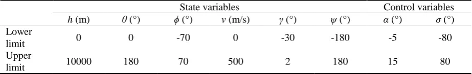
Table 1 shows the lower and upper limit of state variables and control variables.

Table 1. Lower and upper limit of state variables and control variables.

State variables Control variables

h (m) θ (°) ϕ (°) v (m/s) γ (°) ψ (°) α (°) σ (°) Lower

limit 0 0 -70 0 -30 -180 -5 -80

Upper

limit 10000 180 70 500 2 180 15 80

Table 2. Terminal condition of the vehicle.

Terminal state variables Values

hf (m) 200

vf (m/s) 50

γf (°) -10

The goal of this article is to find the maximum range of the gliding vehicle by means of Gauss Pseudo-spectral Method. The gliding vehicle researched in this article has no power system and can achieve the control of velocity by adjusting the flight height or manipulating control surface. [17] During the whole flight, the state of the vehicle is greatly influenced by its attitude, velocity and atmospheric environment at initial position. This article will research the influence of different initial velocities on the trajectory optimization.

Different Initial Velocities

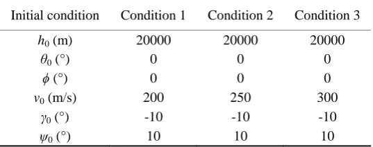
Table 3 lists three different initial conditions and their only difference is velocity. And then, according to different initial conditions, the respective optimization trajectories can be obtained through the program simulation.

Table 3. Initial condition of the vehicle with different velocities.

Initial condition Condition 1 Condition 2 Condition 3

h0 (m) 20000 20000 20000

θ0 (°) 0 0 0

ϕ (°) 0 0 0

v0 (m/s) 200 250 300

γ0 (°) -10 -10 -10

ψ0 (°) 10 10 10

The MATLAB program of trajectory optimization is run and the results are shown from Fig. 1 and Fig. 2. They show the curves of angle of attack and velocity at different initial velocities respectively.

Figure 1. Curves of angle of attack. Figure 2. Curves of velocity.

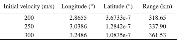
Table 4. Longitudes, Latitudes and ranges at terminal condition.

Initial velocity (m/s) Longitude (°) Latitude (°) Range (km)

200 2.8655 3.6733e-7 318.65 250 3.0386 1.2842e-7 337.90 300 3.2486 1.0835e-7 361.53

It can be seen from Fig. 1 that in the initial stage and final stage of the flight, angle of attack changes violently to accommodate the initial and terminal constraints. However, in the middle of the flight, angle of attack barely changes. It is assumed that the vehicle has already adjusted its altitude and flies smoothly. The simulation results show that angle of attack is about 3.9° in the middle of the flight regardless of the initial state. According to the definition of lift-to-drag ratio and the fitting formulas of lift coefficient and drag coefficient, it can be calculated that when angle of attack is 3.85°, the lift-to-drag ratio of the vehicle reaches its maximum. So, it can be speculated that the gliding vehicle must spend long time flying at the maximum lift-to-drag ratio in order to get the maximum range. Fig. 2 shows that trend of change of velocity is consistent no matter what the initial state is. Also, as long as the initial velocity is constant, other factors have limit impact on the velocity of the gliding vehicle. Table 4 shows ranges under different initial conditions. It can be seen from Table 4 that range of the gliding vehicle changes significantly. It can be inferred that the initial velocity has greater impact on the range of the unpowered gliding vehicle compared to other factors.

Summary

In this article, Gauss Pseudo-spectral Method is used to optimize the trajectory of the gliding vehicle under different initial conditions.

The result shows that in order to maximize the range, it is important to ensure that angle of attack satisfies the maximum lift-to-drag ratio in a long time after recovery for a gliding vehicle. In addition to this, increasing initial velocity is also beneficial to the increase of range.

It can be seen from the research of this article that it has a good effect to solve the problem of trajectory optimization with multi-constraint by using Gauss Pseudo-spectral Method.

Acknowledgement

This research was financially supported by the National Key R&D Program of China under grant No. 2016YFB1200100.

References

[1] N. R. J. Lawrence, S. Sukkarieh, Autonomous exploration of a wind field with a gliding aircraft, Journal of Guidance, Control, and Dynamics, 34(3) (2011) 719-733.

[2] G. Q. Huang, Y. P. Lu, Y. Nan, A survey of numerical algorithms for trajectory optimization of flight vehicles, Science China - Technological Sciences, 55(9) (2012) 2538-2560.

[3] A. S. Nevrekar, A. G. Striz, P. Vedula, Maximum range glide of a supersonic aircraft in the presence of wind, AIAA Aviation Technology, Integration, and Operations, (2012) 1-14.

[4] D. C. Zhang, Q. L. Xia, Q. Q. Wen, G. Q. Zhou, An approximate optimal maximum range guidance scheme for subsonic unpowered gliding vehicles, International Journal of Aerospace Engineering, 2015, (2015) 1-8.

[6] X. Luo, J. Li, Fuzzy dynamic characteristic model based attitude control of hypersonic vehicle in gliding phase, Science China - Information Sciences, 54(3) (2011) 448-459.

[7] P. Lu, Gliding guidance of high L/D hypersonic vehicles, AIAA Guidance, Navigation, and Control, (2013) 1-22.

[8] Y. Xie, L. H. Liu, G. J. Tang, W. Zheng, Trajectory optimization for hypersonic glide vehicle with multi-constraints, Journal of Astronautics, 32(12) (2011) 2499-2504.

[9] G. H. Li, H. B. Zhang, G. J. Tang, Maneuver characteristics analysis for hypersonic glide vehicles, Aerospace Science and Technology, 43 (2015) 321-328.

[10] S. T. I. Rizvi, L. S. He, D. J. Xu, Optimal trajectory and heat load analysis of different shape lifting reentry vehicles for medium range application, Defence Technology, 11 (2015) 350-361.

[11] X. Q. Chen, Z. X. Hou, J. X. Liu, X. Q. Chen, Phugoid dynamic characteristic of hypersonic gliding vehicles, Science China - Information Sciences, 54(3) (2011) 542-550.

[12] C. Y. Dong, Z. Guo, P. B. Zhao, Y. L. Cai, Z. H. Yu, Rapid trajectory optimization for hypersonic reentry vehicle, Journal of Solid Rocket Technology, 38(6) (2015) 757-763.

[13] L. Wang, Q. H. Xing, Y. F. Mao, Reentry trajectory rapid optimization for hypersonic vehicle satisfying waypoint and no-fly zone constraints, Journal of Systems Engineering and Electronics, 26(6) (2015) 1277-1290.

[14] X. D. Yan, S. Lyu, S. Tang, Analysis of optimal initial glide conditions for hypersonic glide vehicles, Chinese Journal of Aeronautics, 27(2) (2014) 217-225.

[15] M. L. Xu, K. J. Chen, L. H. Liu, G. J. Tang, Quasi-equilibrium glide adaptive guidance for hypersonic vehicles, Science China - Technological Sciences, 55(3) (2012) 856-866.

[16] L. Tang Liang, J. M. Yang, F. Y. Chen, Trajectory optimization with multi-constraints for a lifting reentry vehicle, Missiles and Space Vehicles, 1 (2013) 1-5.