Essays in factor based investing

(1)

The London School of Economics and Political Science

Essays in Factor-Based Investing

Tengyu (James) Guo

A thesis submitted to the Department of Finance of the London School of Economics

(2)

Declaration

I certify that the thesis I have presented for examination for the Ph.D. degree of the

London School of Economics and Political Science is solely my own work.

The copyright of this thesis rests with the author. Quotation from it is permitted,

provided that full acknowledgement is made. This thesis may not be reproduced

without my prior written consent.

I warrant that this authorisation does not, to the best of my belief, infringe the

rights of any third party.

(3)

Acknowledgement

Firstly, I would like to express my sincere gratitude to my supervisor Dong Lou for

the continuous support of my Ph.D. study and related research, for his patience,

motivation, and immense knowledge. I would also like to thank Christopher Polk

and Thummim Cho for their supervision, guidance, and help. I could not have

imagined having better advisors and mentors for my Ph.D. study and research.

Besides my advisors, I would like to thank the faculty members that I have

met at LSE: Ashwini Agrawal, Ron Anderson, Ulf Axelson, Elisabetta Bertero,

Mike Burkart, Georgy Chabakauri, Vicente Cu˜nat, Jon Danielsson, Amil Dasgupta,

Daniel Ferreira, Juanita Gonzalez-Uribe, Charles Goodhart, Moqi Groen-Xu, Dirk

Jenter, Christian Julliard, Peter Kondor, Paula Lopes-Cocco, Igor Makarov, Ian

Martin, Martin Oehmke, Daniel Paravisini, Cameron Peng, Rohit Rahi, Domingos

Romualdo, Dimitri Vayanos, Michela Verardo, David Webb, Kathy Yuan, Hongda

Zhong, and Jean-Pierre Zigrand. I benefit from their classes in various courses,

from insightful comments in seminars, and encouragement, but also from the hard

questions which incentivized me to broaden my research and skill set.

My sincere thanks also goes to researchers that I have met outside LSE and

along my studies: Dante Amengual, Manuel Arellano, Pedro Barroso, Samuel

Ben-tolila, Simon Gervais, Jeewon Jang, Liguori Jego, Marcin Kacperczyk, Ralph Koijen,

Daisuke Miyakawa, Omar Licandro, Rafael Repullo, Enrique Sentana, Javier Suarez,

Sunil Wahal, Nancy Xu, and Yu Yuan among the others.

My time at LSE Finance would have been different without many great friends

that I have met during my years as a Ph.D. student. I would like to thank them for

their friendship and support during all these years: Huaizhi Chen, Jingxuan Chen,

Juan Chen, Hoyong Choi, Fabrizio Core, Bernardo De Oliveira Guerra Ricca,

An-dreea Englezu, Jesus Gorrin, Sergei Glebkin, David Haller, Brandon Yueyang Han,

Miao Han, Zhongchen Hu, Jiantao Huang, Shiyang Huang, Bruce Iwadate, Lukas

Kremens, Yiqing Lu, Francesco Nicolai, Olga Obishaeva, Dimitris Papadimitriou,

Jiho Park, Alberto Pellicioli, Marco Pelosi, Poramapa Poonpakdee, Michael Punz,

Amirabas Salarkia, Ran Shi, Simona Risteska, Irina Stanciu, Claudia Robles-Garcia,

Gosia Malgorzata Ryduchowska, Petar Sabtchevsky, Una Savic, Seyed Seyedan, Ji

(4)

Wu, Yun Xue, Xiang Yin, Cheng Zhang and most importantly, Yue Yuan. I also

appreciate the company from friends that I made at different places and the help

from the administration team at LSE Finance department, and in particular, Mary

Comben.

Last but not least, I would like to thank my parents, Jiali and Chenggang, for

giving me life and supporting me as much as they can.

(5)

Abstract

My thesis explores three questions in factor-based investing.

In the first chapter, I study the correlation risk in trading stock market

lies. I propose a simple time-series risk measure in trading stock market

anoma-lies, CoAnomaly, the time-varying average pairwise correlation among 34 anomaanoma-lies,

which helps to explain both the time-series and the cross-sectional anomaly return

patterns. Since correlations among underlying assets determine the portfolio

vari-ance, CoAnomaly is an important state variable for arbitrageurs who hold diversified

portfolios of anomalies to boost their performance. Empirically, I show that, first,

CoAnomaly is persistent and forecasts long-run aggregate volatility of the diversified

anomaly portfolio. Second, CoAnomaly positively predicts future average anomaly

returns in the time series. Third, in the cross-section of these 34 anomaly portfolios,

CoAnomaly carries a negative price of risk.

In the second chapter, instead of studying multiple anomalies in a portfolio, I

focus on one specific anomaly, momentum. I find that the momentum spread

nega-tively predicts momentum returns in the long-term, but not in the following month.

I further decompose the momentum spread into the spread of young or old

momen-tum stocks based on how long the stock has been identified as a momenmomen-tum stock. I

show that the negative predictability is mainly driven by the old momentum spread.

As these old momentum stocks are more likely to be exploited by arbitrageurs, these

findings suggest that momentum is amplified by arbitrage activity and excessive

ar-bitrage destabilizes the asset prices and generates strong reversals.

In the third chapter, I revisit the robust diversification of factor investing and

study the intertemporal consideration of an anomaly investor. Motivated by

Camp-bell et al. (2017), I use vector autoregressions (VAR) and estimate an

intertem-poral CAPM with stochastic volatility for market-neutral investing with the focus

on a portfolio of 34 anomalies. Interestingly, based on my estimation, only the

correlation-induced volatility news carries a significant risk premium, which echos

(6)

List of Tables

1.1 Summary Statistics of CoAnomaly and its Time-series Correlation

with other Measures . . . 53

1.2 Determinants of CoAnomaly and Aggregate Variance . . . 54

1.3 Predictive Regression at Quarterly Level (E.A.R.) . . . 55

1.4 Monthly Sorting with Raw Returns . . . 56

1.5 Monthly Sorting with Benchmark-Adjusted Returns . . . 57

1.6 Monthly Sorting with Daily Raw Returns and Higher Moments . . . 58

1.7 Out-of-Sample Predictability . . . 58

1.8 Predictive Regression with Bootstrap T-stats . . . 59

1.9 Simulation Results for Biased Estimators . . . 60

1.10 Pricing Test of CoAnomaly Risk - Anomaly Assets . . . 61

1.11 Pricing Test of CoAnomaly Risk - Benchmark Assets . . . 62

1.12 Value-Weighted Portfolios Sorted on Predicted CoAnomaly Betas . . 63

1.13 Panel Regression: Partial Correlation of each Anomaly . . . 64

1.14 Regressing the CoAnomaly Shocks and CoAnomaly Levels on Fi-nancial Intermediary Balance Sheet Levels and Shocks . . . 65

1.15 34 Stock Market Anomalies . . . 66

1.16 Predictive Regression at Quarterly Level (E.A.R.) Adjusted with Benchmark . . . 67

1.17 Predictive Regression: Long leg and Short Leg . . . 68

1.18 Predictive Regression: Different Horizons . . . 69

1.19 Predictive Regression: Mean-Variance Efficient Portfolio . . . 70

1.20 Robustness: Correlation between Two Mispricing Factors and 1-month CoAnomaly . . . 71

(9)

2.1 Forecasting one-month Momentum Returns with Momentum spread,

Old momentum spread, Formation gap, Formation Spread, and

Co-momentum . . . 106

2.2 Forecasting Momentum Returns with Momentum Spread and Other Predictors . . . 107

2.3 Forecasting Momentum Spread . . . 108

2.4 Predicting Higher Moments of Momentum: Standard Deviation and Skewness . . . 109

2.5 Momentum Age Distribution . . . 109

2.6 Time-Series Summary Statistics and Correlations among Different Predictors . . . 110

2.7 Forecasting Momentum Returns with Old Momentum Spread . . . . 111

2.8 Comparing the Predictability of Old Momentum Spreads and Other Predictors . . . 112

2.9 Forecasting the Monthly Momentum Strategy Returns in the First Half-Year, the Second Half-Year, and the Second Year . . . 113

2.10 Different Factor Loadings of Old and Young Momentum Portfolios . 114 2.11 Forecasting the Monthly Momentum Strategy Returns in the First Half-Year, the Second Half-Year, and the Second Year . . . 115

2.12 Percentage of Momentum Age in Momentum Stocks. . . 115

2.13 Subsample Analysis: Predicting Momentum Performance with Old Momentum Spread . . . 116

2.14 Out-of-Sample R-squared for Different Predictors . . . 117

2.15 Combo Factor Returns. . . 117

2.16 Combo Factor Returns in 1990-2010. . . 118

3.1 MVE Weights . . . 155

3.2 Out-of-Sample Performance: Returns, Sharpe Ratio and Turnover . 156 3.3 Comparing MVE-Optimized Portfolios with EAR . . . 156

3.4 VAR Estimates for Volatility . . . 157

3.5 Firm-level VAR Estimation . . . 158

3.6 Market-Neutral Asset Pricing Tests . . . 159

(10)

(11)

List of Figures

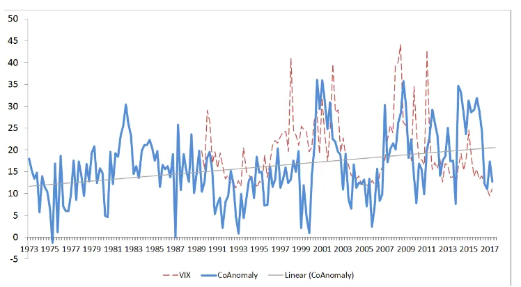
1.1 Time-Series of CoAnomaly . . . 51

1.2 Cumulative Equal-weighted Anomaly Returns after different CoAnomaly periods . . . 52

1.3 Realized versus Predicted Returns: Comparing CAPM versus CAPM + CoAnomaly. . . 72

1.4 Partial Correlation Change around the Publication Year . . . 73

1.5 CoAnomaly (blue solid) and its Bootstrap Standard Error (red dashed, 10000 times) . . . 73

2.1 Different Momentum Strategy Performance . . . 76

2.2 Time-series of Momentum Spread . . . 82

2.3 Momentum Strategy Performance: Old and Young . . . 95

2.4 Cumulative impulse response in Hong and Stein (1999)’s model . . . 99

(12)

Chapter 1

CoAnomaly: Correlation Risk in

Stock Market Anomalies

I propose a simple time-series risk measure in trading stock market anomalies,

CoAnomaly, the time-varying average correlation among 34 anomalies, which helps

to explain both the time-series and the cross-sectional anomaly return patterns.

Since correlations among underlying assets determine the portfolio variance, CoAnomaly

is an important state variable for arbitrageurs who hold diversified portfolios of

anomalies to boost their performance. Empirically, I show that, first, CoAnomaly is

persistent and forecasts long-run aggregate volatility of the diversified anomaly

port-folio. Second, CoAnomaly positively predicts future average anomaly returns in the

time series. Third, in the cross-section of these 34 anomaly portfolios, CoAnomaly

carries a negative price of risk. These return patterns suggest that arbitrageurs take

the time-varying correlation into account and their intertemporal hedging demand

plays an important role in setting asset prices.

JEL-Classification: G11, G23.

(13)

1.1

Introduction

Stock market anomalies are long-short portfolios exploiting stock characteristics

known to predict returns. Since these anomalies generate returns beyond what

standard notions of risk suggest, they have been the subject of a large body of

literature which tries to understand the origins of these anomalies. More recently,

researchers have started to study multiple anomalies jointly; however, they mainly

focus on either reducing the dimensionality of the anomaly space1, evaluating a new

factor given existing factors2_{, or comparing the costs/risks of trading each of these}

anomalies3.

I propose a novel way to understand anomaly return dynamics through the lens

of sophisticated arbitrageurs who trade a diversified portfolio of anomalies. These

arbitrageurs understand the return-volatility trade-off and recognize that the

portfo-lio volatility is time-varying. If cross-anomaly correlation is the main source of news

about current and future volatility of a diversified portfolio of the anomalies, then

the time-varying cross-anomaly correlation arises as a state variable that predicts

the future returns on a diversified portfolio of anomalies in the time series and as a

risk factor that gets priced in the cross-section.

Based on this idea, I propose a simple measure of correlation risk faced by

so-phisticated arbitrageurs. This measure, which I term CoAnomaly, works both as

a predictor of future average anomaly return and as a risk factor that prices the

cross-section of anomaly portfolios.

To construct CoAnomaly, at each point of time, I calculate the average partial

correlation among anomaly returns using daily data within a time window.

Effec-tively, this measure evaluates how much these anomalies comove with each other

across time. I find that CoAnomaly shows time-series persistence and it is not

par-ticularly correlated with major existing risk measures, nor strongly predicted by

other state variables. More importantly, I find that CoAnomaly is the only variable

that can strongly and persistently predict future aggregate variance of the

diversi-fied anomaly portfolio up to one year. On the other hand, aggregate variance or

1_{See Fama and French (1996), Hou et al. (2015), Stambaugh and Yuan (2016), Harvey et al.}

(2016) and Green et al. (2017) among the others.

2_{See Harvey et al. (2016), Feng et al. (2017), and Chinco et al. (2019) among the others.} 3_{See Barroso and Santa-Clara (2015), Novy-Marx and Velikov (2016), Moreira and Muir (2017),}

(14)

average variance of anomalies is quickly mean-reverting and shows no such long-run

predictability. I do not intend to explain the source of correlations among anomalies

at the moment and simply take the time-varying correlation structure as given and

study the asset pricing implications for anomaly investing.

I first explore the time-series predictability of CoAnomaly. As expected, I find

that the na¨ıve equal-weighted anomaly return (E.A.R.) is higher after high CoAnomaly

periods. I focus on E.A.R. for simplicity and I also show that this predictability

ap-plies to the in-sample mean-variance portfolio, which consists of these 34 anomalies.

The predictive regression shows that the quarterly E.A.R. will be 70 basis points

higher following a one-standard-deviation increase in CoAnomaly. This

predictabil-ity shows up robustly after controlling for other predictors, spans from one month to

one year, and does not suffer from the Stambaugh (1999) bias. This predictability

is robust to long and short legs of anomalies as well as different sets of anomalies.

To ease up the interpretation, I provide time-series sorting evidence. For 30% of the

sample period associated with high levels of CoAnomaly, the E.A.R. yields 1.20%

higher returns over the next 6 months, relative to its performance following the 30%

of the sample period associated with low CoAnomaly. The periods with higher

fu-ture anomaly returns do not mean that they are good states for arbitrageurs, as I

find that the future standard deviation of E.A.R. is higher and its skewness is more

negative after high CoAnomaly periods. Moreover, I find that the predictive power

is stronger in the recent half of my sample period, as the E.A.R. performance

differ-ence between high CoAnomaly periods and low CoAnomaly periods almost doubles

(from 1.20% to 2.36%). This sample period coincides with the period of fast

emer-gence and growth of professional asset managers. Furthermore, the predictability is

even more pronounced when I focus on the periods when quantitative equity hedge

funds suffer a low return (a proxy for high risk aversion), which is consistent with

the risk-return trade-off story from the perspective of these arbitrageurs. I also

con-duct a battery of robustness checks to make sure my results would not be driven by

several possible mechanisms.

In the cross-section, I find that the innovation of CoAnomaly carries a negative

price of risk. The negative sign of risk premium suggests that higher CoAnomaly

(15)

check two sets of testing assets: the anomaly set including the 34 anomaly portfolios,

which are used to calculate the CoAnomaly measure, and a standard set which

includes equity portfolios sorted by size, book-to-market, momentum, and industry,

as well as the cross-section of Treasury bond portfolios sorted by maturity. The

price of risk is significant, and its magnitude is consistent across test portfolios and

specifications. On average, the quarterly risk premium associated with one unit

of the CoAnomaly beta is around -5%. In other words, investors demand lower

expected returns for portfolios that covary positively with CoAnomaly, since these

portfolios effectively provide hedges against the CoAnomaly risk. This finding is

consistent the with the recent event, ‘quant meltdown’ in August 2007, documented

by Khandani and Lo (2007) and Khandani and Lo (2011), in which they argue that

this hard period for quantitative investors is accompanied by high correlation among

their strategies. The fact that the correlation risk also gets priced in a broader set of

portfolios (industry portfolios and bonds) suggests the large presence of these asset

managers in different financial markets. Furthermore, the loadings on CoAnomaly

innovation help explain the cross-sectional return dispersion across these portfolios.

That said, my single factor does not fully explain the cross-section of anomaly returns

as large intercepts are left unexplained. I further construct CoAnomaly beta sorted

portfolios from stock level based on their estimated real-time CoAnomaly betas.

I find large dispersion in adjusted returns that line up well with the post-ranking

CoAnomaly betas.

My paper contributes to the literature in two aspects. First, I show that both the

time-series and cross-sectional return dynamics of stock market anomalies can be

partially explained by taking a portfolio view of these anomalies. This view stems

from the perspective of portfolio managers in quantitative equity hedge funds who

are betting on these anomalies, goes back to the basic trade-off between risk and

return, and studies the time-varying risk of trading these anomalies as diversified

portfolios. By focusing on the correlations among these anomalies that vary across

time, I provide evidence supporting the basic risk-return trade-off relationship in

anomaly asset prices. Moreover, this also sheds light on the understanding of the

volatility-managed portfolios by highlighting the importance of the correlation risk.

(16)

contrast, I study these anomalies jointly in a portfolio and show that it is the

comovement among these anomalies that plays a key role in evaluating the risk.

Second, CoAnomaly gives a better understanding of the investing behaviors of

the fast-growing sophisticated institutional investors, as I find that the time-series

predictability is stronger in the recent half of the sample, which coincides the period

with rapid growth in asset management industry4_{. Moreover, the predictability is}

even more pronounced when these arbitrageurs are suffering low returns,

presum-ably inducing a higher risk aversion and making their trade-off incentives stronger.

On the other hand, since the CoAnomaly risk mechanically affects the investment

opportunity of these arbitrageurs, the hedging demand on this risk feeds back into

asset prices and a negative risk premium of CoAnomaly shows up in the

cross-sectional dispersion of average asset returns. My findings suggest that, first, these

arbitrageurs understand that the risk they face is time-varying and know how to pick

certain assets to hedge it; and second, their impacts to the market are substantial

so we can observe these return patterns from asset prices.

1.2

Related Literature

The exploration of stock market anomalies starts from the early testing on CAPM

and the empirical failure of a single market factor witnesses the explosion of

iden-tifying stock market anomalies by academics as well as by practitioners. Finance

researchers find it difficult to reconcile them with standard asset pricing models,

and several streams of approaches have been proposed to understand them:

ex-post factor models, principal component analysis, behavioral stories, intermediary

asset pricing, etc. On the practitioners’ side, it is not just the arbitrageurs strictly

chasing market neutrality, but also investors whose portfolio deviates from the

mar-ket portfolio are loading on certain strategies to some extent. Most recently, the

Exchange-Traded Fund (ETF) industry also started issuing factor-based ‘smart beta’

products, and both long-term investors and retail investors are investing in these

assets, hoping to boost their Sharpe ratio (see Cao et al. (2018)). There has always

been a debate about whether these anomalies represent true risk-adjusted excess

4_{Schwert (2003) and Chordia et al. (2011) find evidence that arbitrage activity on anomalies}

(17)

returns or whether they are compensation for omitted risk factors. I take no stand

on this issue and simply adopt the consensus interpretation of the market-neutral

quantitative equity investors who believe these anomalies do generate alphas with

respect to the market portfolio. Though concerns have been raised on whether there

are too many anomalies (see Hou et al. (2017)) or whether they can survive

trans-action costs (see Novy-Marx and Velikov (2016)), Martin Utrera et al. (2017) find

that transaction costs increase the number of significant characteristics due to the

canceling-out of transaction costs when combining and rebalancing characteristics.

It has been documented that these anomalies are indeed exploited by

sophisti-cated investors. Hanson and Sunderam (2013) use the short interest to show that

the amount of capital devoted to value and momentum, the two most prominent

strategies, has grown significantly since the late 1980s; McLean and Pontiff (2016)

find that anomaly returns are lower after publication. Because of the sophisticated

nature of these large and professional agents, some researchers argue that they are

aware of the (endogenous) systemic risk and will internalize the impact of their

be-havior. Koijen and Yogo (2015) find that most cross-sectional variation in stock

returns is contributed to retail investors instead of large asset managers.

Mean-while, there are also concerns about their roles and impacts, as Stein (2009) points

out that crowding and leverage can impair market efficiency and argue that capital

regulation may be helpful in dealing with the latter problem. Both theoretical work

and empirical evidence show this destabilizing effect of arbitrageurs, see Vayanos

and Woolley (2013) and Lou and Polk (2013).

When it comes to trading these anomalies, a proper risk measure is necessary to

access the cost and benefit. However, recent literature has documented the failure

in proper pricing of variance risk in finance as well as in macroeconomics.

Dew-Becker et al. (2017) find it was costless on average to hedge news about future

variance at horizons ranging from 1 quarter to 14 years between 1996 and 2014, and

only unexpected, transitory realized variance was significantly priced. Berger et al.

(2017) find that shocks to uncertainty have no significant effect on the economy, even

though shocks to realized stock market volatility are contractionary according to a

wide range of VAR specifications. On the other hand, as assets comove together, the

(18)

and hence the future risk premium. Correlation Risk is studied pervasively. Pollet

and Wilson (2010) show that the average correlation between daily stock returns

predicts subsequent quarterly stock market excess returns since the market risk is

determined by the individual risks and the correlation among them. They start

from a measurement error issue of aggregate risk and show that changes in true

aggregate risk may nevertheless reveal themselves through changes in the correlation

between observable stock returns. However, I take a portfolio view of anomalies

from the arbitrageurs and show that the average correlation is an important state

variable, which acts as both a predictor in the time-series and a priced risk in the

cross-section. Driessen et al. (2009) study the different exposures to correlation

risk between index options and individual stock options and find that correlation

risk exposure explains the cross-section of the index and individual option returns

well. Buraschi et al. (2010) provides a theoretical model in which the degree of

correlation across industries, countries, or asset classes is stochastic. Buraschi et al.

(2013) find that the ability of hedge funds to create market-neutral returns is often

associated with significant exposure to correlation risk, which helps explain the large

abnormal returns found in previous models, and they also estimate a significant

negative market price of correlation risk. Adrian and Brunnermeier (2016) propose

a measure for systemic risk: CoVaR, the value at risk (VaR) of financial institutions

conditional on other institutions being in distress.

However, most research on the correlation risk mainly focuses on the correlation

risk in the aggregate stock market. This paper takes a novel perspective of looking at

the anomaly space from the scope of a portfolio manager chasing market neutrality

and studies the time-series predictability and cross-sectional pricing together. As a

closely related research, Stambaugh et al. (2012) find that investor sentiment

posi-tively predicts anomaly returns and argue that short-sale impediments contribute to

their finding as their effect concentrates on the short legs of anomalies. My result is

different from theirs in the sense that the predictability of CoAnomaly shows up for

both long legs and short legs, which is in line with the basic trade-off between risk

and expected return. Sotes-Paladino (2017) explores the optimal dynamic

invest-ment problem when mispricing assets are correlated, in which he considers a constant

(19)

time-variation in the correlation structure.

1.3

CoAnomaly

1.3.1

Data and Anomaly Construction

To construct the stock market anomalies, I use the stock return data from the

Center for Research in Security Prices (CRSP). The accounting data is taken from

Compustat - Capital IQ, and short interest data from Supplemental Short Interest

File of Compustat - Capital IQ. Since I use quarterly accounting information with

validReport Date of Quarterly Earnings (RDQ) starting from late 1971 to construct

some anomalies, my main sample period starts in 1973 and ends in 2017. As my

later analysis does not depend on a balanced panel, I extend my main sample period

back to 1963 as a robustness check in the appendix (with anomalies which do not

require RDQ information), which generates consistent results.

The hedge fund index data is taken from the Hedge Fund Research website. The

HFRI® Indices are broadly constructed indices designed to capture the breadth of

hedge fund performance trends across all strategies and regions. I use the Equity

Market Neutral Index (HFRIEMNI), which studies the quantitative equity funds

and dates back to the beginning of 1990. Mispricing factors data is taken from

Stambaugh’s website5_{. TED rate data is downloaded from the website of Federal}

Reserve Bank of St. Louis.

I consider a combined set of 34 stock market anomalies6 _{studied in the}

litera-ture. For each anomaly, I compute the time-series of monthly value-weighted (VW)

returns on a long-short self-financed portfolio over the period 1973m1-2017m12. I

use the NYSE breakpoints for the anomaly characteristics to sort all stocks traded

on the NYSE, AMEX, and NASDAQ. To make sure my results are not driven by

micro-cap stocks and other microstructure issues, I exclude stocks with prices below

$5 per share or are in the bottom NYSE size decile. I closely follow Stambaugh

5_{I thank Robert Stambaugh for providing the daily mispricing factors data.}

6_{32 anomalies are following the}_{the data library (click here)}_{for Novy-Marx and Velikov (2016),}

(20)

et al. (2012), Novy-Marx and Velikov (2016) and Cho (2017) to construct

anoma-lies, and the full set of anomalies is shown in appendix’ Table 1.15. I also normalize

all anomalies to make sure they have positive abnormal returns so that arbitrageurs

would hold a positive position on them.

1.3.2

CoAnomaly Calculation

I first construct value-weighted anomaly portfolios by sorting stocks into deciles

based on their anomaly characteristics available at the end of month t-1. Here,

I follow the standard procedure in the literature by using the NYSE breakpoints

for the sorting and the anomaly portfolio is longing the top decile and shorting

the bottom decile7. I construct both daily and monthly anomaly portfolios, and

I also use the cumulative monthly anomaly returns in a quarter as the quarterly

returns for the anomaly. After obtaining all the anomaly portfolios, I then compute

partial correlations using daily returns for each anomaly portfolio with respect to

the equal-weight of other anomaly portfolios8. CoAnomalyLS is the average partial

correlation for long-short anomaly portfolios. Short-leg CoAnomaly (CoAnomalyS₎

is theaverage partial correlation for the bottom deciles of all anomalies, and long-leg

CoAnomaly (CoAnomalyL_{) is the} _average _{partial correlation for the top deciles of}

all anomalies. Lou and Polk (2013) use this procedure to proxy the crowdedness of

momentum arbitrage activity; however, I use this to measure the correlation risk.

CoAnomaly_tLS = 1

N

X

n=1

partialCorrt(retLSn , ret LS

−n|M ktRf)

| {z }

Average partial correlation for anomalyn

with respect to all other anomalies−n

= 1

N

X

n=1

ρLS_n,₋_n,

CoAnomalyS_t = 1

N

X

n=1

partialCorrt(retSn, retS−n|M ktRf) = 1

N

X

n=1

ρS_n,₋_n,

7_{I adjust the signs of anomaly characteristics so that the outperforming stocks are always on}

the top deciles (example: small stocks and value stocks).

8_{There is concern about nonsynchronous trading as in Frazzini and Pedersen (2014), but the}

(21)

CoAnomaly_tL= 1

N

X

n=1

partialCorrt(retLn, ret L

−n|M ktRf) = 1

N

X

n=1

ρL_n,₋_n,

where N is the number of total test anomalies, retLSn (/S/L) is the daily return of

the long-short(/short-leg/long-leg) portfolio for anomaly n, and retLS−n(/S/L) is the

equal-weight daily return of long-short(/short-leg/long-leg) portfolios for all test

anomalies apart from anomaly n.9

The correlation is partial in the sense that I control for market exposure when

computing this correlation to purge away any comovement in anomaly returns

in-duced by the market. Two practical facts can justify this consideration. First,

most arbitrageurs (like hedge funds) who are the main traders and exploiters of

these anomalies are chasing market neutrality; and in general, the market betas on

portfolio level are fairly stable and can be predicted and hedged well.

I use the look-back period for three months, which means the CoAnomaly measure

at the end of June is constructed using daily returns in April, May, and June.

However, my main results are robust to other specifications, including the

one-month look-back window (with stronger effects). The CoAnomaly time series can

also be calculated by calculating the summation of the non-diagonal elements in

the correlation matrix for all anomalies, which generates the same results in the

qualitative sense.

1.3.3

Time Variation and Determinants of CoAnomaly

(Insert Table 1.1)

Table 1.1 reports the summary statistics of the CoAnomaly measure. I find that

CoAnomaly for long-short anomaly portfolios is mainly driven by the short leg.

CoAnomaly behaves quite differently for the long legs and the short legs, with a

negative correlation. In terms of magnitude, the short leg CoAnomaly is larger than

long leg CoAnomaly, which could be justified by the following: 1) Apart from size

9_{I also calculate the average pairwise partial correlation of the anomalies by averaging the}

(22)

anomaly, most anomalies tend to have large firms on the long leg and small firms

on the short leg, so a larger price impact should be expected on the short leg than

on the long leg, and 2) arbitrageurs have a relatively higher trading presence than

other investors on the short legs and they tend to trade all these assets

simulta-neously. Note that CoAnomaly is not driven by the average correlation between

the constituents in the aggregate market by Pollet and Wilson (2010) as they are

mildly correlated. Later, I also include the average correlation in the market in my

predictive regression and find no effect.

I also check the contemporaneous correlations among different CoAnomaly

mea-sures and other market indices in the second half of my sample since some of them

are only available from the 1990s. I find that CoAnomaly is related to the market

realized variance and the VIX index, which suggests that CoAnomaly is related to

the risk in the market, but the comovement is not entirely matched. This pattern

can be seen in Figure 1.1 as well. The figure also shows an increasing trend in

CoAnomaly, which may be linked to the growth of sophisticated investors in the

last few decades. The market excess returns, TED rate, market liquidity level, and

equity neutral hedge fund index do not have a particularly strong correlation with

the CoAnomaly measure.

I also find that CoAnomaly is highly correlated with the correlation between two

mispricing factors as in Stambaugh and Yuan (2016), who argue that most stock

market anomalies can be explained by these two mispricing factors. Finally, the short

leg CoAnomaly exhibits positive correlation with sentiment index10 _{from Baker and}

Wurgler (2006), which is consistent with Stambaugh et al. (2012) and suggests that

the high sentiment from overoptimistic retail investors may cause excess correlation

on overpriced assets.

Predicting CoAnomaly

CoAnomaly_t=a+b×CoAnomaly_t₋₁+X

p

mp×Controlsp,t−1+t×Trend+et. (1.1)

(Insert Table 1.2)

(23)

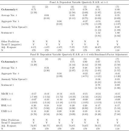
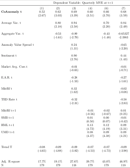
In panel A of Table 1.2, I conduct a predictive analysis of CoAnomaly to find the

potential determinants of the time-varying CoAnomaly. I find that all CoAnomaly

measures are fairly persistent and have a positive trend (except for the long leg

CoAnomaly). I run extra regressions of long-short CoAnomaly on various

vari-ables with a one-quarter lag. The investor sentiment appears to be the only

con-sistently strong predictor of CoAnomaly11_{. As the standard deviations of other}

non-CoAnomaly regressors are normalized to 1, a one-standard-deviation increase

in market sentiment predicts around a 3 percent increase in CoAnomaly in the

eco-nomic magnitude. Apart from sentiment, none of the coefficients for other predictors

shows persistent significance, which includes market excess return, average liquidity,

TED rate, and Equity Market Neutral Index (HFRIEMNI)12.

One final observation is that the trend of CoAnomaly does not go beyond the

linear trend as the F-test for R-squared yields a value of 1.59, which indicates that

the increase in R-squared is not significant on adding more polynomials, as shown by

specification [4] in panel A of Table 1.2. From this point, unless explicitly addressed,

when I talk about CoAnomaly, I refer to the long-short CoAnomaly13_.

1.3.4

Risk Measure: Variance or Correlation?

Predicting the Aggregate Anomaly Variance The variance of a diversified

portfolio, which serves as the traditional measure of the risk, is determined by both

the average variance of the constituent assets and the average correlation among

them14_{. I focus on a na¨ıve portfolio by investing in these anomalies with equal}

amounts, and I term the return asEqual-weighted Anomaly Return (E.A.R.), which

is the simple equal-weight mean return of 34 stock market anomalies. DeMiguel

11_{However, I do not include the investor sentiment in the VAR for later analysis as Jeffery}

Wurgler argues in his website: Do not use these series for measuring changes in sentiment (e.g. sentiment(t)-sentiment(t-1)) due to lag structures, among other considerations, as these are low-frequency levels indicators.

12_{From a crowdedness of arbitrage capital perspective, this is not surprising considering that}

while high arbitrage capital (lower TED rate, larger higher market, and hedge fund return, lower volatility or higher liquidity) would induce more capital allocated in these anomalies, it is also possible that arbitrageurs trade more frequently when they are facing capital constraints. Both of these mechanisms may increase the comovement among assets. Given these effects are mixed, I do not overinterpret the signs at the moment.

13_{Empirical results remain qualitatively the same if I use the short leg CoAnomaly.} 14_{Consider a simple case: a portfolio with N symmetric assets, when N is large:} _σ2

p = N ×

(_N1)2_σ2_{+ 2}_×N(N−1) 2 (

1 N)(

1

(24)

et al. (2007) show that many in-sample optimized techniques fail to beat the na¨ıve

1/N rule out of sample in terms of Sharpe ratio, certainty-equivalent return, or

turnover. Later, I also extend my analysis to the in-sample mean-variance efficient

portfolio for robustness check.

In the first part of panel B of Table 1.2, I report the results of regressing the

realized aggregate variance of the equal-weighted anomaly returns (E.A.R.) on the

contemporaneous CoAnomaly and the average realized variance of single

anoma-lies. The aggregate variance of the Equal-weighted Anomaly Returns (E.A.R.) is

measured as the variance of daily returns within a given quarter. Average realized

variance is equally averaging the realized daily variances for the 34 stock market

anomalies in the same quarter. The results show that both CoAnomaly and the

av-erage variance contribute to the variance of the E.A.R., and these two components

capture almost all of the time-series variation in the E.A.R. aggregate variance (as

the R-Squared reaches 80%).

The remaining parts of panel B of Table 1.2 conduct predictive regression for the

aggregate variance of E.A.R. by using CoAnomaly, average variance, and aggregate

variance of E.A.R with lags up to four quarters. However, for average variance

and aggregate variance, the predictability quickly dies out after 2 quarters as the

R-squared dropped from around 50% for one-quarter lag to below 10% for above

two-quarter lags. On the contrary, CoAnomaly robustly and persistently explains

20% to 10% of the aggregate variance variation, for lags from one to four quarters.

These results (both the coefficients and the R-squared) clearly show that CoAnomaly

is the only component that maintains a strong predictive power across the one-year

period, and they also support the choice of CoAnomaly as a risk measure.

Economic Intuition Pollet and Wilson (2010) presents a stylized model to show

that the average correlation among assets, but not the average variance, is positively

related to the risk premium. They show that the risk premium is given by:

Et[rs,t+1]−rf,t+1+ ρ_tσ2_t

2 =

γ βt(1−θt)

ρ_tσ2_t − γ

βt(1−θt)

θtσ2t, (1.2)

where rs,t+1 is the return on the stock market, rf,t+1 is the risk-free rate, ρt and

(25)

beta of stock market on the aggregate wealth portfolio, θt is the proportion of the

stock market risk component to the total risk for a single stock.

As shown in the equation, the relationship between risk premium and average

variance is not clear; however, the relationship between risk premium and the average

correlation is positive because the stock market is part of the aggregate wealth

portfolio. The reason behind this is that if the changes in the stock market variance

are orthogonal to the risk in aggregate wealth portfolio, then such changes in stock

market variance should be offset by changes in the covariance of the stock market

with the rest of the aggregate wealth portfolio, holding the risk of aggregate wealth

portfolio constant.

From another point of view, if single assets share common components from the

aggregate portfolio, the increase in volatility of this common component will, first,

drive up the volatility of single assets, and second and more importantly, induce

stronger comovement among these single assets. When the aggregate portfolio

can-not be measured perfectly, the volatility of an alternative pseudo-aggregate portfolio

can be a bad proxy for the aggregate risk. However, the correlation effect between

single assets remains robust.

In the market-neutral investment setting, these stock market anomalies constitute

only a subset of the whole investment universe of the sophisticated investors, which

is a perfect scenario that fits Roll (1977)’s critique. As argued in Pollet and Wilson

(2010), if the Roll (1977)’s critique is important, the variance may be weakly

cor-related with the aggregate risk and subsequent excess returns. Following the same

logic, the variance in these anomalies may provide contaminated information about

the risk of their aggregate portfolio.

Why not covariance? Standard portfolio theory states that the risk of a single

asset evaluated with respect to a diversified portfolio is measured by the covariance

between the asset and the portfolio. However, in the case of stock market anomalies,

I argue that CoAnomaly is a better measure than the covariance to proxy the risk:

to access the covariance, a benchmark portfolio is required, which is unrealistic in

the case of sophisticated institutional investors. Unlike the standard macrofinance

models normally assuming that long-term investors hold the aggregate market, the

(26)

stock market, to fixed-income, derivatives, and even to real estates and antiques.

On the other hand, even if the composition of the portfolio is identified, the exact

weight on each asset (strategy) is still unknown. Meanwhile, leverage is widely used

by these professional institutional investors and they manage their leverage ratio

across time and strategies. This effect also obfuscates the estimation of weights in

different strategies/anomalies. Therefore, in the case of sophisticated arbitrageurs,

a benchmark portfolio like the market portfolio cannot be observed, hence the

co-variance measure lacks a clear definition to measure the risk.

However, if single assets share common components from the aggregate portfolio,

the increase in volatility of this common component will induce stronger comovement

among these single assets. This effect on comovement also justifies my choice of using

the average correlation to calculate the CoAnomaly measure.

1.4

Time-Series Predictability of Anomaly Returns

Suppose an investor invests in a bundle of risky assets. Ceteris paribus, the increase

in the average return correlation among all these assets will make the optimal

port-folio riskier by increasing the variance, and the rational investor will ask for a higher

return on holding these assets as compensation. Given the sophisticated nature of

arbitrageurs, the risk-return trade-off is expected to hold in the anomaly investment

setting.

1.4.1

Predictive Regression

I first conduct the following predictive regression analysis to see whether CoAnomaly

can predict future anomaly returns:

E.A.R.t+1 = a+b×CoAnomalyt+t×Trend

+X

p

mp×Other.Predictorsp,t (+

X

j

×βjBenchmark.F actorst+1) +et+1.

(1.3)

(27)

In panel A of Table 1.3, I regress the equal-weighted anomaly Returns (E.A.R.) in

the next quarter on the observables incurrent quarters using non-overlapping data.

I also include a trend variable in all regressions, which turns out to carry a significant

negative coefficient, and this is consistent with recent findings of the return decay

in these anomalies (see McLean and Pontiff (2016)). The standard deviations of

all predictive regressors are normalized to 1. Column (1) shows that CoAnomaly

is a strong predictor of the E.A.R. and it alone with the trend can explain 8.1

percent of the time-series variation of the E.A.R.. Columns (2) and (3) show that

the predictive powers of the average variance and aggregate variance of anomalies

are negligible, consistent with recent findings of the weak or negative predictability

of variance measures (see Barroso and Maio (2018)). The economic magnitude of

CoAnomaly predictability on the E.A.R. is more than 70 basis points per quarter

given the one standard deviation change in CoAnomaly. Columns (4) and (5) include

both CoAnomaly, the average variance, and the aggregate variance of E.A.R., and

they show that only the average correlation predicts future returns. Next, I control

for the anomaly value spread and the sentiment. Anomaly value spread is the

average value spread for all anomalies, which is the difference in weighted average

log book-to-market ratio between the long legs and short legs. As Cohen et al.

(2003) argue the value spread must predict future returns, profitability and/or the

persistence of valuation levels following the firm-level decomposition by Vuolteenaho

(2002). Stambaugh et al. (2012) find that anomaly returns are higher following high

investor sentiment constructed by Baker and Wurgler (2006) and I find that the

sentiment has a strong predictive power. Nevertheless, the predictive power of my

CoAnomaly survives with statistical significance, albeit with a smaller scale. In the

last specification, the predictability remains strong after controlling other potential

predictors, including TED spread (TED), market excess return, market average

correlation, and E.A.R..

In panel B of Table 1.3, I report the benchmark-factor-adjusted regression results

as a clean-up test. I want to make sure that the time-variation in average anomaly

returns that CoAnomaly predicts is not driven by the benchmark factors as many

papers15_{have argued that there are risk factors behind these factors. I can also tease}

15_{See Fama and French (1992), Campbell and Vuolteenaho (2004), Zhang (2005), Lettau and}

(28)

out the part of variation associated without any ‘premium’ like size factor, in which

alpha-seeking arbitrageurs will have less interest. Here I use Carhart (1997)

four-factor model as a benchmark, and my results are robust to different specifications,

including a single market factor, Fama-French three-factor model, and Fama-French

five-factor model. Once the returns are adjusted with contemporaneous benchmark

factors, CoAnomaly shows much stronger predictability. Note that the E.A.R.

load-ings on benchmark factors are consistent with literature: in general, (overpriced)

stocks in the short legs tend to be small stocks with higher market beta, which

results in negative loadings on both market factor and size factor; and anomalies

tend to load on value and momentum as Asness et al. (2013) point out.

In nontabulated results, I also show that my results are robust, albeit with smaller

magnitudes, when including two contemporaneous mispricing factors in Stambaugh

and Yuan (2016). Note that their study is focusing on explaining the cross-sectional

dispersion of anomaly returns by measuring their loadings on the two mispricing

factors; however, my result is focusing on the time-variation of anomaly returns. The

smaller magnitudes after controlling two mispricing factors, together with the fact

that E.A.R. is strongly loading on these two factors, suggest that the time-varying

returns of the two mispricing factors can also be explained, at least partially, by

CoAnomaly.

Anomaly Set Specification To make sure my results are robust to anomaly

specifications, I conduct the same analysis for two different sets of anomalies: 23

anomalies studied in Novy-Marx and Velikov (2016) (NMV) and 11 anomalies

stud-ied in Stambaugh et al. (2012) (SYY) separately. CoAnomaly, E.A.R., and other

anomaly-relevant measures are constructed with only these two sets, respectively.

The results are reported in the appendix, and I find that the predictability of

CoAnomaly is robust. However, I also find that the market sentiment has a

rel-atively stronger predictive power in the original anomaly set studied in Stambaugh

et al. (2012).

Sample Periods I check if my results are robust to 1) extending the main sample

period back to 1965, or 2) excluding the most recent financial crisis in 2008. The

(29)

prices. As for the stock market anomalies, there has been some research on the

different behaviors during these periods: Daniel and Moskowitz (2016) show that

momentum strategy lost close to 50 percent following the 2008 turmoil.

Separate Long Legs and Short Legs Moreover, I show that CoAnomaly

pre-dicts future returns on anomalies for both their long legs and short legs, which is

more aligned to the risk-return trade-off story. The results can be found in the

appendix (see Table 1.17). My results are different from Stambaugh et al. (2012), as

they find that their predictability is concentrated on the short legs and argue that

this is consistent with a combination of short-sale impediments and market-wide

sentiment.

Different Horizons The predictive power of CoAnomaly is also robust for shorter

or longer horizons (see Table 1.18 in the appendix). However, the regression result

for 6-month E.A.R. is the strongest in terms of both coefficients and adjusted

R-squared, which is not surprising considering there is more noise in short run, and

the predictability will die out in the long run owing to the time-varying nature of

CoAnomaly. This also helps to partially alleviate the concern of spurious regression

raised by Ferson et al. (2003), since they argue that if the expected returns are

per-sistent, there is a risk of finding a spurious relation between the return and an

inde-pendent, highly autocorrelated lagged variable. Here, I show that the predictability

is strongest for 6 months, and the CoAnomaly measure has an autocorrelation

coef-ficient around 0.5 for 3 months, so in the 6-month window, the persistence level of

CoAnomaly is relatively low, which violates the ‘highly autocorrelated’ condition of

the spurious regression concern.

Mean-Variance Efficient Portfolio I also check the predictability for a

mean-variance efficient (MVE) portfolio consisting of these 34 anomalies, though I do not

focus my analysis on this ex-post efficient portfolio, which neither researchers nor

arbitrageurs know ex-ante. I compute the MVE portfolio weights by maximizing the

sample Sharpe ratio with respect to a zero-beta rate equal to 0, based on the

in-sample average returns and covariance matrix. Sophisticated arbitrageurs will hold

(30)

risk-return trade-off to show up for the MVE portfolio. Consistent with my conjecture,

Table 1.19 in the appendix shows that the predictability for the MVE portfolio is

similar to that for the E.A.R..

1.4.2

Sorting in Time-series

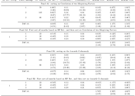
(Insert Table 1.4)

To ease up the interpretation, I also provide evidence by sorting all months in

the time series. As shown in Panel A of Table 1.4, all months are sorted into three

groups based on CoAnomaly in month t. All sorting variables are detrended16 _and

the time-series sorting uses 30% and 70% as breakpoints.

First, I show that higher past CoAnomaly does predict higher future CoAnomaly.

Note that the persistence in CoAnomaly is a necessary condition for the

predictabil-ity under the risk-return trade-off mechanism. I then check the returns of equal

weighting the long-short returns of all anomalies from the next month (t+1) to half

of a year (t+6). There is a monotonic and persistent pattern across groups, as high

CoAnomaly months are followed by high average returns on anomalies. On

aver-age, the difference in returns between following a high CoAnomaly and following a

low CoAnomaly (Diff 3-1) is 120 basis points in the following 6 months, which is

economically large and statistically significant.

I split my full sample periods, from 1973Q1 to 2017Q4, into two halves: 1)

pre-1994 and from 1973Q1 to 1993Q4, and 2) post-pre-1994 and from pre-1994Q1 to 2017Q4.

As I turn to the second half of my sample (Panel B1 of Table 1.4), the predictability

is much stronger in both economic and statistical senses, as illustrated graphically

in Figure 1.2. This fact could be partially justified by the explosion of finding stock

market anomalies and the emergence of sophisticated institutional investors since

the early 90s. This split is also robust to different cutting points.

Double-sorting I further check whether this pattern will hold under different

market conditions for anomaly investors. I expect the asset pricing pattern from

the risk-return trade-off will be stronger when the investors are more risk-averse.

16_{Detrending means that I am not biasing my analysis to the front or tail of my sample periods.}

(31)

Given the fact that hedge funds are the main players in trading these anomalies, I

use the quantitative equity hedge fund returns (later HF Ret.) to proxy the

risk-aversion of these arbitrageurs. Among Hedge Fund Research Indices, I choose the

HFRI Equity Market Neutral Index, HFRIEMNI17_{, which is the average return of}

all market-neutral quantitative equity funds in their database, to proxy the shocks

to these arbitrageurs. Therefore, I first sort all months based on the hedge fund

returns in month t, and then within each group, I sort on the CoAnomaly level. As

shown in Panel B1 of Table 1.4, the two sorting variables, column HF Ret. t, and

column CoAnomaly t do not show any particular relationship, so if I conduct the

double sorting independently, the results remain unchanged qualitatively.

Panel B2 of Table 1.4 shows the results of the double sorting. The predictability is

much stronger and more significant in the distress periods of hedge funds especially

in the short-run. Although the evidence is by no means definitive, it is consistent

with the possible explanation that due to various reasons, including the withdrawal

of capital by investors, hedge fund managers show higher risk aversion after poor

returns so the risk-return trade-off pattern in asset prices is stronger.

The main advantage of using the HFRIEMNI is that it is a direct measure of the

shocks to the arbitrageurs who are mainly trading stock market anomalies, which

is better than using the average returns on all anomalies as a proxy to the shocks

to the arbitrageurs because I cannot assume that arbitrageurs are betting these

anomalies consistently across time. There is a large body of literature documenting

the timing ability of different anomalies (e.g. Cohen et al. (2003) for timing value,

Lou and Polk (2013) and Barroso and Santa-Clara (2015) for timing momentum,

Moreira and Muir (2017) for timing an extensive set of factors based on their realized

volatility). Barroso et al. (2017) directly test the behavior of institutional investors

with 13F institutional holdings data, and find that these investors actually decrease

their loading on momentum before momentum crash, which rejects the idea that

17_{On their website, they state that ‘Equity Market Neutral strategies employ sophisticated}

(32)

momentum crashes relate to institutional crowding. However, in results not shown

here, I also did the same test using the equal-weighted return on all anomalies as

a proxy of shocks to arbitrageurs and find similar patterns, but with less statistical

significance.

Control for Benchmark Factors Consistent with predictive regression, the

re-sults are stronger if I control for contemporaneous benchmark factors (a single

mar-ket factor and Carhart (1997) 4-factor model), as shown in Table 1.5. In

non-tabulated results, I find that my results are robust if I use post-1990 as the second

half of my sample, as the hedge fund index starts from 1990.

(Insert Table 1.5)

Evidence from Daily Returns and Higher Moments I report the summary

statistics of the daily raw returns of E.A.R.. The average daily raw returns show

similar patterns on the monthly level. The standard deviation of the E.A.R. is

also high after high CoAnomaly periods. More importantly, I find that the E.A.R.

returns tend to left-skewed more strongly following high CoAnomaly periods. In

the second sample period, the daily raw returns of E.A.R. show higher standard

deviations as well as stronger crash risks.

These empirical patterns clearly show that though the average (first moment) of

E.A.R. returns are higher after high CoAnomaly period, the risks (higher moments)

in trading anomalies are also higher. This pattern echoes the ‘Unwind

Hypothe-sis’ analyzed in Khandani and Lo (2011), in which they observed large correlation

and crash in returns of long-short equity strategies during the ‘quant meltdown’ in

August 2007.

(Insert Table 1.6)

Other Robustness Checks In the appendix, I explore other drivers that may

affect my results: principal component analysis of these anomalies, small and high

idiosyncratic stocks driving results, too many anomalies and lack of dimension,

different CoAnomaly calculation window, and anomalies sharing same stocks. None

(33)

1.4.3

Out-of-Sample Tests and Econometric Issues

Here I conduct out-of-sample (OOS) tests and also explore two econometric issues

that might undermine the validity of my results, and I find evidence that the

pre-dictability of CoAnomaly is robust.

Out-of-Sample Tests In the out-of-sample tests, I compare the predictive power

between the historical sample mean and the predictive regressions. For both

meth-ods, the forcast for quarter t only uses information up to quartert−1. The

out-of-sample statistics are standard in the literature18following McCracken (2007), Welch

and Goyal (2008) and Huang (2015).

One predictive regression of quarterly E.A.R. returns on CoAnomaly produces

an out-of-sample R-square of 2.16%. This contrasts with the results of other

pre-dictors for E.A.R. as well as the usual negative OOS R-squares of similar predictive

regressions for the market excess return.

(Insert Table 1.7)

Generated Regressors The standard errors in the above predictive regression

re-quire a caveat because the regressor CoAnomaly is generated from the daily anomaly

returns. To make sure this extra layer of noise does not undermine my main result,

I conduct a double-layer block bootstrap based on Djogbenou et al. (2015) and the

detailed process is described in the appendix. Table 1.8 reports the t-stats with

Newey and West (1987) correction and the t-stats with bootstrap standard errors.

The differences between these two are marginal and my results remain significant

robust.

(Insert Table 1.8)

This is not surprising since effectively, the CoAnomaly measure is calculated quite

precisely with high-frequency data used in the process. In the appendix, I show that

the standard errors in the CoAnomaly measure are relatively small compared to its

own time-variation.

18R2= 1−M SEA M SEN,R

2_{= 1}₋₍₁_−R2₎ T−k−1

T−k−p−1, ∆RM SE=

√

M SEN−

√

M SEAandM SE−F =

(T −k)M SEN−M SEA

M SEA , where M SEA and M SEN are the mean square errors of the predictive

(34)

Biased Estimators As Stambaugh (1999) points out: when a rate of return is

regressed on a lagged stochastic regressor, the OLS estimator will be biased if the

innovations of the dependent variables and the innovations of the regressors are

correlated. A simple illustration of the Stambaugh (1999) bias (omitting means):

rt+1 =b×predt+et+1

predt+1 =φ×predt+ut+1.

(1.4)

In small-sample AR(1) regression, the estimate ˆφtends to be downward biased. If

Cov(et+1, ut+1)<0, then the coefficient in the predictive regression will be inflated,

as

E(ˆb−b) = Cov(et+1, ut+1)

V ar(ut+1) E

( ˆφ−φ).

In my setting, there can be a potential problem since CoAnomaly is proxying the

risk. If the latent risk gets higher, the innovation in the CoAnomaly measure will

increase, and in the meantime, the assets will suffer a contemporaneous bad shock

as the future discount rate increases due to higher risk. This mechanism may lead

to a negative relationship between et+1 and ut+1.

To make sure my results do not suffer from this bias, I estimate a restricted

vector autoregression (VAR(1)) for the E.A.R. and CoAnomaly. I am interested in

the covariance between two shocks as well as the variance of the CoAnomaly shock.

E.A.R.t+1 =a+b×CoAnomalyt+et+1

CoAnomalyt+1 =c+d×CoAnomalyt+ut+1.

(1.5)

By estimating a VAR with only E.A.R. and CoAnomaly (both are detrended first

to avoid complication, and CoAnomaly is also normalized that standard deviation

equals to 1), I find that the estimated E.A.R. shockset+1and CoAnomaly shocksut+1

are almost uncorrelated, with the correlation coefficient being equal 0.08. Moreover,

I also follow Baker et al. (2006) and conduct a Monte Carlo simulation under the

null, i.e., there is no predictability (b = 0). In the last column of panel B in

Table 1.9, I show that across several specifications, the probability that the simulated

coefficient,b, is higher than my estimated coefficient is always less than 0.01%. This

(35)

the Stambaugh (1999) bias.

(Insert Table 1.9)

1.5

Price of Risk in Cross-Sectional Asset Prices

CoAnomaly positively predicts both higher volatility and higher returns on these

stock market anomalies; in other words, it forecasts changes in the distribution of

future return (investment opportunity). If there are some assets that comove with

CoAnomaly, I would expect sophisticated investors to use them as hedges.

Here I follow the procedure of Fama and MacBeth (1973) and Adrian et al. (2014)

to conduct a standard asset pricing test of whether CoAnomaly is priced in the

market. I use the simple detrended-AR(1) innovation etin the CoAnomaly measure

(the error terms in the specification (1) in Panel A of Table 1.2) as the shock here

for simplicity although my results are robust to other alternative specifications.

CoAnomaly_t=a+t×Trend +b×CoAnomaly_t−1+t (1.6)

In the first step, based on different pricing models that I check, I regress the

excess returns on the different factors (including the innovations of CoAnomaly t)

to get their risk exposures or betas:

Re_i,t =ci+

X

j

βi,jfj+ei,t, t= 1,2, ..., T for all i.

Then I run a cross-sectional regression of time-series average excess returns,

E[Rei,t], on risk factor exposures βb_i estimated from the last step:

E[Rei] =λ0+ X

j

c

βi,jλj +ξi.

By doing this, the risk premia of different factors λj as well as the zero-beta rate

λ0 are calculated. Here, I assume that all assets have constant betas on different

(36)

1.5.1

Price of Risk in Anomaly Portfolios

I first use the 34 long-short stock market anomalies as test portfolios. As they are

traded by anomaly arbitrageurs, I expect CoAnomaly to be priced among them.

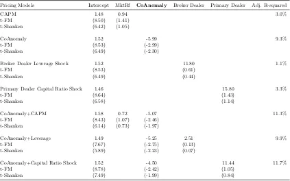
(Insert Table 1.10)

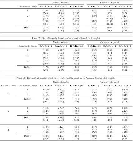
Table 1.10 shows that CoAnomaly carries a significant and negative price of

risk. The negative sign of CoAnomaly risk means that investors are willing to

accept a lower average return if the asset positively comoves with CoAnomaly. In

other words, assets with a positive loading on CoAnomaly will give a lower average

return because these assets tend to do well in high CoAnomaly periods, providing

hedges against the CoAnomaly risk. This is consistent with the empirical fact that

CoAnomaly is a strong and persistent predictor of future aggregate variance for

these anomalies: so the increase in CoAnomaly implies higher aggregate volatility,

hence worse investment opportunity. This result echoes the finding in Driessen et al.

(2009). As both returns and CoAnomaly are measured in percentage, the economic

magnitude is that, given other things equal, one unit increase in the CoAnomaly

beta will lower the quarterly return of the asset by around 5%.

In the last column of Table 1.10, I also show the adjusted R-squared in the

cross-sectional regression, which represents how much the cross-sectional dispersion

of average returns among these anomaly portfolios can be explained by different

loadings on the factors. The single market factor only explains 3%, and once it

is augmented with CoAnomaly, they can explain 11.3% of the return dispersion.

This is a good performance given two facts: first, the test portfolios are 34 stock

marketanomalies which are famous for being difficult to price, and second,

contem-poraneous return benchmarks only explain the dispersion with a similar proportion

(7.8% for Fama and French (1996) three-factor model and 13.8% for Carhart (1997)

four-factor model in nontabulated result).

I also control for two intermediary asset pricing factors: leverage of securities

broker-dealers from Adrian et al. (2014) and equity capital ratio of primary dealers

He et al. (2017). Both of these studies find a positive price of risk of the shocks

to financial intermediaries. I find that CoAnomaly maintains significant pricing

(37)

positive) risk premium.

Note that there are large intercepts left for these anomaly portfolios.

Conse-quently, the standard Chi-square test of pricing errors gets rejected overwhelmingly.

However, pricing all assets is not the main purpose of the exercise here. All

evi-dence shown here is to support the fact that the CoAnomaly risk gets priced among

anomalies themselves. Moreover, it also helps explain the cross-sectional return

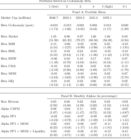
dispersions partially, as shown in the top two figures in Figure 1.3.

(Insert Figure 1.3)

1.5.2

Price of Risk in a Standard Set of Portfolios

I also use the standard set of test portfolios, which are the commonly studied equity

and government bond portfolios: 25 Fama-French size-value portfolios, 10

momen-tum portfolios, 5 industry portfolios, and 6 treasury bond portfolios sorted by

ma-turity19. Five industry portfolios are included to make sure that my results are not

driven by the strong factor structure within size, value and momentum portfolios,

as suggested by Lewellen et al. (2010).

(Insert Table 1.11)

The point estimates of risk premia are different across specifications, but they

stay in a stable range and are slightly larger than the estimates in anomalies: On

average, one unit of loading on CoAnomaly generates -8% percent risk premium

per quarter. In nontabulated results, I find that CoAnomaly risk premium gets

subsumed to zero if I include all size, value and momentum factors together, which

is not surprising since most test portfolios are based on the characteristics behind

these factors and hence have a strong factor structure that