2016 International Conference on Artificial Intelligence and Computer Science (AICS 2016) ISBN: 978-1-60595-411-0
Survey for Image Magnification and Parameter Problem Issues
Based on Gauss Distribution Function
Chun-jing LI
1,*and Xian-xian CHEN
21Department of Mathematics, Tongji University, Shanghai 200092, China
2Department of Mathematics, Tongji University, Shanghai 200092, China
*Corresponding author
Keywords: Gauss distribution function, Image magnification,Parameter problem.
Abstract. In this paper, we do image magnification based on Gauss Distribution Function on Kriging Method. Firstly, we process the digital image matrix is to continuous block matrices. Secondly, we simulate and enlarge the matrices with Gauss Distribution Function. Finally, we compare the quality
of enlarged images between Gauss and Multi-Quadric method on average Euclidean distance
. Wefigure out Gauss Function does better both in gray images and color ones. Besides, we find out that the most suitable parameter value c is 1.305 in gray image and 1.28 in color image. Above all, we enlarge figures with better function and find out the most suitable parameter values in this method.
Introduction
Under the development of computer and Internet technologies, a lot of difficult issues and research problems have been solved gradually. Image processing has made great progress as well. Growing demand for digital image information has prompted the development of image processing technology. It has been made a great progress in this area, some algorithms even applicable systems have been exploited. [1]But most are limited to the theoretical discussion, which can’t put into practice.
In the paper, we choose the method of Gauss distribution function to enlarge the image. On one hand, we want to find out which method can gain smoother image [2]. On the other hand, we want to figure out the parameter problem issues based on Gauss distribution function.
Image Enlargement Process
Radial Basis Function
Radial basis function is a function basis, which is obtained by a unary function in Euclid distance. It is a function of
:R R, in domainxRd. It’s like
x c
x c
. Its linear combinationgenerates the function spaces, which is called the radial basis function space derived from[3]. As long as
xj are not the same,
xxj
are linearly independent under certain conditions.Then a set of base is formed in the subspace of radial basis function space. So when
xj get all thevalues inR,
xxj
and its linear combination can approximate any function.Definition
1 The definition of variable convolution of radial function
x and
x [4] :
*d
x
y xy dy
(1)Definition
2 Radial basis function
x
x is positive definite. If for all two different pointsets 1, , d
n
x x R , matrix
, j k
x j k n
A x x
Frequently-used radial basis functions are as follows[5]:
(1)The method of Kriging Gauss distribution function:
exp
2 2
r c r
(2) (2)The Multi-Quadric distribution function:
2 2
r c r
(3) (3)The Dickon thin plate spline:
r r22k dk dlogr when d is an even numberr when d is an odd number
(4)
In this paper, we do enlargement based on Gauss distribution function:
exp
2 2
r c r
.
Magnified by 2 × 2 Continuous Block Matrix
We transfer interpolation in digital image processing into radial basis interpolation problem. A set
of data points sized M × N can be showed as
31
, , n
i i i i
x y f R [6].Imagef x y
, can be expressedthrough the function relationship betweenxandy.
The method of Gauss distribution function:
r exp
c r2 2
. Image f x y
, can be expressedthrough the function relationship between x and y. So, the function is defined by[8]
2
2
2
1* , n j exp j j
j
f x y c x x y y
(5) Satisfy the condition
2
21
* , exp
n
j j j
j
f x y
c x x y y
(6) And the K should be nonsingular[7].
2
2 2 ,, , 1, 2, ,
j j
i j
K
xx yy c i j n
The image matrix sized200 200 is processed2 2 discrete and continuous block matrices (refer
with: Fig.1), then we simulate the lock matrices and do enlargement. Finally we amalgamate the matrices. Method for continuous block matrices is used for in following experiments.
Figure 1. Discrete block and Continuous block.
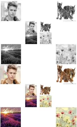
Experiment I—Results of Gray and color Image on New Method and the Comparison
[image:3.612.173.439.63.504.2]
Figure 2. Different Kinds of Pictures by the Experiment.
Comparison of Multi-Quadric and Gauss Function
We grab the different
to do comparison. Am n , for the original gray image. Bm n , the numericalmatrix for images that’s magnified k times. Eigenvalues of A are changed according to
size, 1A 2A A
p
,p
min
m n
,
. So as B. We give average Euclidean distance:
2
|| ||
1, 2, ,
B A
i i i p
p
(7) The smaller
is, the better the magnified image is.Discussion about properties on
Table 1. The comparison of the quality of the images on different radial basis functions.
Multi Quadric
Gauss1 1.3061 1.306
2 2.7829 2.7829
3 2.8263 2.8262
4 2.4832 2.4831
5 3.0804 3.0802
6 2.8368 2.8367
Conclusion I
Method of Gauss function is better on the quality of magnification.
Parameter Issue Problem of the Gauss Distribution Function of Gray and Color Image
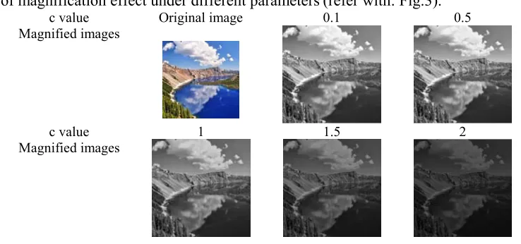
In order to quantify the influence of parameters on the magnified images, We choose a blue sea image, changes of magnification effect under different parameters(refer with: Fig.3).
c value Original image 0.1 0.5
Magnified images
c value 1 1.5 2
Magnified images
[image:4.612.160.445.84.187.2]
Figure 3.Different magnified images under different parameters.
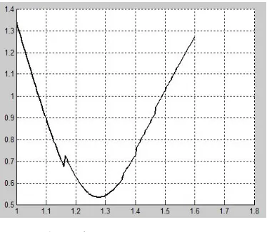
It is apparent that when c is smaller than about 1, images are quite clear and in good quality. But when c is bigger, the corresponding images have serious mosaic phenomenon. Make up p = 100, we make a table on the variation results (refer with: Table 2) and draw a picture with much more points (refer with: Fig.4). Points of axis of abscissas are parameters, points of axis of ordinates are the values of
.Table 2. The comparison results.
c 1.01 1.03 1.05 1.07 1.09 1.11 1.13 1.15 1.17
1.5373 1.4598 1.391 1.3114 1.2316 1.1537 1.0751 1.0655 0.9956
c 1.19 1.21 1.23 1.25 1.27 1.29 1.31 1.33 1.35
0.9283 0.864 0.8044 0.7523 0.7067 0.6682 0.679 0.679 0.6722
c 1.37 1.39 1.41 1.43 1.435 1.440 1.445 1.450 1.455
0.6776 0.6848 0.697 0.7131 0.7193 0.726 0.7337 0.7427 0.7482
In order to quantify the same to the color images, we also choose blue sea image (refer with: Fig.5). Here the points of axis of abscissas are the values of parameters and the points of axis of ordinates are the values of average Euclidean instances (refer with: Fig.6). Points of axis of abscissas are parameters, points of axis of ordinates are the values of
. [image:4.612.118.487.278.451.2]Figure 4.The relevance of c and
.c value Original image 1.01 1.31
Magnified images
c value 1.41 2 3
[image:5.612.213.400.66.218.2]Magnified images
Figure 5.Different magnified images under different parameters.
Figure 6. The relevance of c and
.In order to find out the more exact parameter c value to get the best quality of the function, a new index is defined like:
4
| i j| 10
Q (8)
Here
i,j are corresponding with ,c ci jremain to consider.Conclusion II
From the results, along with the increase of the value of c to about 1.305 for gray images (1.28 for
[image:5.612.213.400.437.600.2]is obvious. When c is bigger than about 1.305(1.28), along with the increase of c,
is increasing as well. That is to say, in this area, when c is bigger and bigger, therefore, the quality of the image is worse.This is because the smaller error is produced in the process of interpolation of f x y
, which gets the function f*
x y, , the value of c determines the size of the error in the proportion of the wholefunction. The greater of the value of c, the smaller of the proportion of error is when c is small than about 1.305(1.28).
However, when c is bigger than about 1.305(1.28 for color images), the error is increasing with the increase of c. Finally it is found that the most suitable range is c is about 1.305(1.28 for color images).
Summary
In this paper, based on Gauss Distribution Function, we do enlargement on gray and color images. The enlarged images have a high quality. Compared with the former method based on Multi-Quadric function, this method is better. Besides, based on the average Euclidean distance and limitationQ, the most suitable parameter value c is 1.305 in gray images and 1.28 in color ones.
Acknowledgement
This work is supported by the Key Project of NSFC Guangdong Joint Foundation under Grant No. U1135003 .We thank the sponsors and the support of the School of Mathematical Science of Tongji university.
References
[1] Chunjing Li, Jinwu Liu, A method of image magnification based on radial basis function, Journal of Information and Computational Science 13 (12)(2015) 1-7.
[2] X.Y. Fang, X.P. Wei, H.F. Teng, Study on data processing and animation reconstruction based on facial motion capture, Journal of Dalian University of Technology (2010) 109-112.
[3] Adil Masood Siddiqui, Asif Masood, Muhammad Salem, A locally constrained radial basis function for registration and warping of images, Pattern Recognition Letters 30 (2009) 377-390. [4] Zongmin Wu, Radial basis function. Scattered data fitting and the massless deviation equation, Journal of Engineering Mathematics 19 (2) (2002) 10-11.
[5] M.D. Buhmann, Radial Basis Functions, Theory and Implementations, Cambridge University Press 2004 (11-27).
[6] Lazzaro D., Montefusco L., Radial basis function for the multivariate interpolation of large scattered data sets, Journal of Computational and Applied Mathematics 140 (1/2) (2002) 521-536. [7] Narcowich F., Ward J., Norm of inverses and condition numbers for matrices associated with scattered data, J. Approximation Theory 64 (1991) 69-94.