A New Method of Origin Destination Survey Using License Plate Recognition by Recursive Traffic Zone Division

2016 International Conference on Computer, Mechatronics and Electronic Engineering (CMEE 2016) ISBN: 978-1-60595-406-6

A New Method of Origin-Destination Survey Using License Plate

Recognition by Recursive Traffic Zone Division

Dong-fang FAN

and Xiao-li ZHANG

1_{Transportation Management College, Dalian Maritime University, Linghai Road, Dalian, Liaoning}

116026, China

2_{China Academy of Transportation Sciences (CATS), No.240 Huixinlin, Chaoyang District Beijing}

100029, China

Keywords: Origin-Destination matrices estimation, License Plate Recognition (LPR), Traffic zone

division, Recursive method.

Abstract. This paper proposes a new method of using License Plate Recognition (LPR) for Origin-Destination (OD) survey. LPR has shown many advantages in OD estimations such as lower average acquisition costs than other OD surveys, more information extracted from vehicles passing by LPR devices etc. We recommend a recursive method of traffic zone division as to flexibly divide traffic zones by network conditions or practical needs. In order to improve the speed of license plate matching process, we adopt an index structure of LPR database by the coding of license plates. Two important special OD cases, having-O-and-no-D and no-O-and-having-D are handled to supplement OD information by expanding the searching space-time scopes in database. The methodology is perfectly validated by an example of OD survey for a road network in CBD of Beijing.

Introduction

Origin-Destination(OD) survey is a key component of transportation planning, Traffic control and management system etc. Traditional acquisition methods of OD matrices could be divided into two categories: OD sample survey and OD matrices estimation. In recent years, the OD estimation by Automatic Vehicle Identification (AVI) and License Plate Recognition (LPR) is widely used with continuous collection of dynamic OD information via LPR devices (Yasui, 1995; Makigami, 1995; Van, 2007; Constantinos, 2007, Chao, 2009), making up for the shortage of insufficient information collection by loops.

Constantinos et al. (2007) indicated that LPR technologies facilitate the collection of useful data, such as point-to-point travel time and sub-path flows.

Yasuo(2002) showed a formulated least squares model and yields to linear transportation of

partial observed OD matrices. However, due to the quantity limitations of LPR cameras and their

locations limitation, the proposed methodology restricts the application to a corridor part of a network. Van (2007) proposed a Bayesian updating procedure which allows the presence of random error in traffic counts and misrecognition at LPR stations, dealing with the inequality constraints in an appropriate statistical manner. Chao (2009) contributed an O-D matrix survey sample in Shanghai City with dynamic data collection of different time intervals.

there are several problems that remain unsolved yet at present:

(1) The process of LPR is time-consuming and, often leads to biased results (Doblas, 2005). Especially, in cases of large network or traffic zones with many access roads, more surveys are needed to distinguish vehicles traveling by different directions between zones.

(2) Many trips beginning during time interval t may not be completed until some future time intervals. It means vehicles “disappear” without any destination points. Therefore, the OD information for time t is incomplete because of the partly matching of LPR in a real-time situation (Dixon, 2002).

requirement. The approach could reduce OD survey complexity effectively. We can get a series of OD matrices between sub-zones to sub-zones or traffic zones to sub-zones.

(2) The application of indexed searching technology and database has shorten the matching time of license plates greatly. This is the main advantage to heighten the matching speed.

(3) After LPR, we can decrease the unmatched proportion of license plates via collating, merging, and comparing the OD matrices by enlarging the space-time searching scopes.

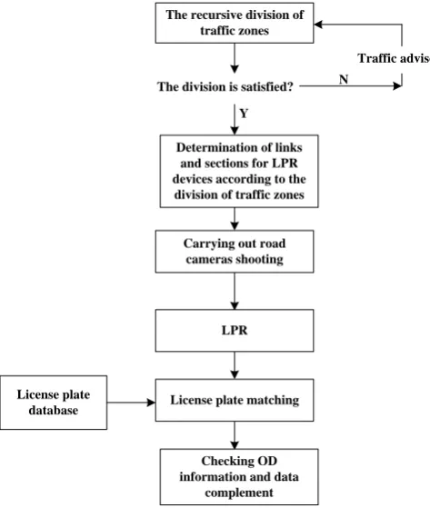
The Operational Process of OD Survey by LPR

The process of OD survey by LPR is organized as follows. The recursive division of traffic zones makes it easy for traffic advisors to judge when to stop the division process. LPR data from different sections of links in the network is stored and accessed by indexed LPR database. We can adjust OD matrices with different time intervals to supplement the incomplete matrices derived from partly license plates matching. The whole system is shown as below.

The recursive division of traffic zones

The division is satisfied?

Traffic advisor N

Y

Determination of links and sections for LPR devices according to the

division of traffic zones

Carrying out road cameras shooting

LPR

License plate matching License plate

database

Checking OD information and data

complement

Figure 1. The process of OD survey by LPR.

The Main Processes and Subsystems in OD Survey by LPR

The Recursive Division of Traffic Zones

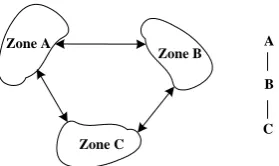
In traffic controls or planning, sometimes, we may need to learn a series of OD matrices of different areas such as traffic zone-subzone, zone-zone, subzone-subzone. Subzones may be obtained by several cutting steps of a large-scale area. The division of traffic zones has no fixed ways, depending on traffic survey requirement or advisors. A traffic zone could be either a wide region like Chaoyang district in Beijing or restricted in a commercial center or a residential area like the CBD area in Beijing. Furthermore, if we continue to divide it, the sub-zone could be even a traffic hub like Beijing Railway Station which congregates railway, subway and bus stations. In order to make the definition of traffic zones and the relationship between traffic zones and OD matrices clear, we firstly take some following examples.

Zone A Zone B Zone C A B C

Figure 2. The division of traffic zones A, B, C.

We can get an OD matrix M:

M=           CC CB CA BC BB BA AC AB AA (1)

If traffic zone A is divided into two sub-zones A1 and A2. We can get four zones of A1, A2, B, C. The inner relations between A1 and A2 are not considered.

A1 A2

B

C

A

A1 A2 A

A1B A2B AB

A1BC A2BC ABC

Figure 3. The traffic zones after A is divided into two sub-zones A1 and A2.

We can get three OD matrices M1, M2, M3.

(2) The boxed elements in M2 and M3 are not consistent with the corresponding ones in M1, while others the same.

In the following, we continue to divide traffic zone B into two sub zones B1 and B2.

A1 A2

B1 B2

C

A

A1 A2 A

A1B1 A1B1C A1B2 A1B2C A2B1 A2B1C A2B2 A2B2C AB1 AB1C AB2 AB2C A1B A1BC A2B A2BC AB ABC

Figure 4. The traffic zones after B is divided into two sub-zones B1 and B2.

M1=           CC CB CA BC BB BA AC AB AA

, M2=

          CC CB CA C B B B A B C A B A A A 1 1 1 1 1 1 1 1 1 1 1 1 , M3=           CC CB CA C B B B A B C A B A A A 2 1 2 2 2 1 2 1 2 1 1 1

, M4=

          CC CB CA BC BB BA C A B A A A 1 1 1 1 1 1 , M5=       C B B B A B C A B A A A 1 1 1 2 1 2 1 2 2 2

, M6=

M7=           CC CB CA BC BB BA C A B A A A 2 2 2 2 2 2

, M8=

          CC CB CA C B B B A B AC AB AA 1 1 1 1 1 1 , M9=           CC CB CA C B B B A B AC AB AA 2 2 2 2 2 2 (3)

It indicates that we can get exponential number of OD matrices with the continuous divisions of traffic zones. Parts of the elements of OD matrices in the former division could be used in the OD surveys of the latter. This is the main advantage of recursive division method of traffic zones.

Locations of Sections and Links for LPR Cameras.

After the division of traffic zones, we need to determine the locations of sections or links for LPR cameras. In order to get the precise OD information, we usually put LPR cameras near the borders between two zones. We use Fig.5, a network of CBD area in Beijing for our description.

The whole network is about 2.2 square kilometers, composed by seven arterial roads and a section of an expressway named the East 3rd Ring Road, one of the busiest roads in Beijing. We firstly divide the area into two zones A and B so as to get a better understanding of the sub-network and the impacts from zone A to zone B at different time intervals.

Sometimes, it is very necessary to capture the impact degrees of some certain areas in the origin zone A to the destination zone B, therefore we divide the origin zone A into three sub-zones A1, A2 and A3 and divide the destination zone B into three sub-zones B1, B2 and B3 according to the road structure of CBD district as Fig.6 and Fig.7 shown. The OD matrix between the sub-zones is shown as Formula 4.

Chaoyangbei Road

Chaoya_{ng Road}

D o n g d a q ia o R o a d J in to n g x i R o a d J in to n g d o n g R o a d Guanghua Road Jianguo Road E a st 3 rd R in g R o a d Guomao Bridge A B Chaoyangbei Road Chaoya_{ng Road}

D o n g d a q ia o R o a d J in to n g x i R o a d J in to n g d o n g R o a d Guanghua Road Jianguo Road E a st 3 rd R in g R o a d 1# 5# 3# 7# 12# 15# Guomao Bridge A1 A2 A3 B1 B2 B3 2# 6# 4# 11# 8# 9# 10#

13# 14#

Figure 5. A road network of CBD in Beijing. Figure 6. The sub-zones after division.

A

A1 A2 A3 A

A1B1 A1B2 A1B3 A1B A2B1 A2B2 A2B3 A2B A3B1 A3B2 A3B3 A3B AB1 AB2 AB3 AB

Figure 7. OD matrix after zones A and B are divided into three parts respectively.

(4) The boxed OD elements are the ones we mostly want to know in the network, while the others have less meanings.

St(v,u) is the set of vehicles passing by section v, and re-appearing in section u within the time interval t.

St(v1)⊙St(v1)=(St(v1)∪St(v1))- (St(v1)∩ St(v1)) (5) Count(S) means the number of elements in set S.

As an example, we introduce the calculation operations of the OD element of A1B1. The operation steps of others are similar.

In time interval t, the vehicles passing by section 7# of zone B1, marked as St(7#), contain three parts of vehicles: the first case represents the passing vehicles from 2# or the upstreams of the East 3.rd Ring Road. A second case is the vehicles from roads outside of A1. The last one represents the vehicles produced by zone A1 that we want to know. As the former two cases of vehicles are not

produced by zone A1 actually, we should move them away from St(7#).

(1) Find all the entrances to zone A1 and B1, labeled as 1#, 3#, 4#, 5#, 6# and 2# respectively. The next operations are carried out to remove all the vehicles produced by zone B1 or outside areas of zone A1 and re-appeared among the set of vehicles passing by the destination section 7#.

Therefore, the left vehicles have the same origin zone A1, which is also the init OD of A1B1. The

following is the detailed operations.

(2) Eliminate all the passing vehicles whose license plates are recognized by section2# and re-appear at section 7# within time interval t at the destination zone B1. This can be expressed as

St(7#)- St(2#,7#).

(3) Continue to eliminate all the passing vehicles produced out of A1, whose license plates are recognized at sections 1#, 3#, 4#, 5#, 6#, and re-appear at the section 2# in the time interval t. This could be expressed as St(7#)- St(2#,7#)- St(1#,7#) St(3#,7#)- St(4#,7#)- St(5#,7#)- St(6#,7#).

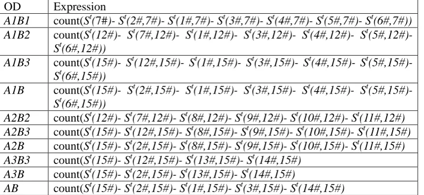
After the above two steps, the number of the elements of the left set of St(7#) is the init OD from A1 to B1, namely count(St(7#)- St(2#,7#)- St(1#,7#) St(3#,7#)- St(4#,7#)- St(5#,7#)- St(6#,7#)). All the OD expressions are shown as Table 1.

Table 1. The OD expressions.

OD Expression

A1B1 count(St(7#)- St(2#,7#)- St(1#,7#)- St(3#,7#)- St(4#,7#)- St(5#,7#)- St(6#,7#)) A1B2 count(St(12#)- St(7#,12#)- St(1#,12#)- St(3#,12#)- St(4#,12#)- St(5#,12#)-

St(6#,12#))

A1B3 count(St(15#)- St(12#,15#)- St(1#,15#)- St(3#,15#)- St(4#,15#)- St(5#,15#)- St(6#,15#))

A1B count(St(15#)- St(2#,15#)- St(1#,15#)- St(3#,15#)- St(4#,15#)- St(5#,15#)- St(6#,15#))

A2B2 count(St(12#)- St(7#,12#)- St(8#,12#)- St(9#,12#)- St(10#,12#)- St(11#,12#) A2B3 count(St(15#)- St(12#,15#)- St(8#,15#)- St(9#,15#)- St(10#,15#)- St(11#,15#) A2B count(St(15#)- St(2#,15#)- St(8#,15#)- St(9#,15#)- St(10#,15#)- St(11#,15#) A3B3 count(St(15#)- St(12#,15#)- St(13#,15#)- St(14#,15#)

A3B count(St(15#)- St(2#,15#)- St(13#,15#)- St(14#,15#)

AB count(St(15#)- St(2#,15#)- St(1#,15#)- St(3#,15#)- St(14#,15#)

From Table 1, we could find some repetitive elements in the ODs, such as St(15#) has appeared

seven times when the destination zones are B or B3; St(12#,15#) has appeared three times when the destination zones are B3; St(3#,15#) has appeared twice when the OD pairs are A1B and A1B. The repetition of the elements makes it easy to simplify the calculation as much as possible.

Example of OD Surveys

LPR was carried out off-line after the shooting was finished. Because of normal traffic and weather conditions, the correct rate of LPR is over 95%, so there is no need to discuss the influence of the wrong LPRs to OD surveys. The use of index technology for license plate matching has improved the computational speed to approximately 12s for every OD within one time interval. In the following, we will give the analysis for OD surveys from three points of view in detail.

● The average OD matrices and traffic flow proportions from sub-zones of A to sub-zones of B ● The OD comparisons with different time intervals at working and no-working days

● Special cases analysis of having-O-and-no-D and no-O-and-having-D.

The Average OD Matrices and Traffic Flow Proportions from Sub-zones of A to Sub-zones of B

In this section, we give an overview of OD matrix between sub-zones of A and B via averaging the ODs of the observed seven days.

M=                             578 , 17 142 , 7 3 553 , 7 2 375 , 3 1 067 , 5 3 067 , 5 3 3 0 2 3 0 1 3 932 , 6 2 299 , 3 3 2 091 , 4 2 2 0 1 2 921 , 7 1 165 3 1 738 , 4 2 1 375 , 3 1 1 AB AB AB AB B A B A B A B A B A B A B A B A B A B A B A B A (6)

It could be seen that there are about 17,578 vehicles from zone A into zone B during 7:00~19:00, about 1400 vehicles/hour, bringing a large traffic burden on the East 3rd Ring Road. The sub-zones A1, A2 and A3 contribute 7,921, 6,932 and 5,067 vehicles respectively on arterial roads like Chaoyangbei Road, Chaoyang Road, Guanghua Road and Jianguo Road. These roads are mostly over 2,500 vehicles/hour in rush hours, among the busiest arteries in CBD area of Beijing.

The OD Comparisons with Different Time Intervals at Working and No-working Days

The traffic patterns are quite different between working and non-working days. It also influences the OD distributions. We select ODs of A1B, A2B, A3B and AB to have a comparison them within different time intervals. Figure 7 and Figure 8 show the results of the OD flows between the working days and non-working days.

2000 4000 6000 8000 10000 12000 14000 16000 18000 20000 22000

A1B A2B A3B AB Mon Tue Wed Thu Fri 0 2000 4000 6000 8000 10000 12000 14000 16000 18000 20000

A1B A2B A3B AB Sat

Sun

Figure 7. ODs of A1B, A2B, A3B and AB

in the working days. Figure 8. ODs of A1B, A2B, A3B and AB in non-working days.

Special Cases Analysis of having-O-and-no-D and no-O-and-having-D

Having-O-and-no-D and no-O-and-having-D are two special cases reflecting the time-varying feature of OD. Having-O-and-no-Ds are those vehicles that have been attracted from areas outside origin zones into zone A within time interval t, but could not be recognized at any other zone within time interval t and neither half an hour later. So the quantity of having-O-and-no-Ds may be not only an evaluating indicator of the traffic activity levels of the origin zone, but also a reference of the balance between the having-O-and-no-Ds and no-O-and-having-Ds. Furthermore, we could learn more information about having-O-and-no-Ds by the contribution proportions of the traffic volumes of the connecting roads to sub-zones of A.

On the contrary, no-O-and-having-Ds are those vehicles that are recognized at destination zones, but we are not sure where they have come from? We could give an approximate estimation of the contribution proportions of sub-zones A1, A2 and A3 to zone B. After the steps of the OD data complement in part 3.4, we could draw the conclusion that A1 has the largest contribution 41.71% to B, and A2, A3 accounts for 30.82% and 27.45% respectively.

Conclusion and Further Research

In this paper, a method of using License Plate Recognition (LPR) technology is developed to origin-destination surveys. With the requirements of better traffic planning and control to learn more information of ODs between zones, sub-zones and zones or sub-zones and subzones, we propose a recursive traffic zone division to flexibly divide traffic zones by network conditions and practical needs. The application of indexed structure of LPR database by the coding of Chinese license plates has improved the calculation speed greatly in the matching and accessing process with the license plate database.

In a real open network, there should be inevitably incomplete information of OD matrices, typically for two special cases: having-O-and-no-D and no-O-and-having-D. For non-taxi vehicles, we utilize the group of OD matrices with the same origin zones or destination zones at different time intervals to fill the vacancies in OD matrices. Except for taxies, which have no fixed routes, we try to expand the time searching scopes of LPR database to resolve the problem. A full analysis of OD survey example in an area of a road network in CBD of Beijing has been made from three points of view which focus on the overview of OD matrices between sub-zones in the observed days, OD fluctuations between working and no-working days and the special cases analysis of having-O-and-no-D and no-O-and-having-D.

References

[1] Chao, G..P., 2009. Ma, W.M., Li, Y. Origin-destination survey by license plate recognition. China ITS Journal. 2, 76-78

[2] Constantinos, A., Moshe, Ben-akiva., Haris, N.K. 2004. Incorporating automated vehicle identification data into origin-destination estimation. 37-44.

[3] Dixon, M.P., 2002. Real-time OD estimation using automatic vehicle identification and traffic count data. Computer-aided civil and infrastructure engineering 17, 7-21.

[4] Doblas, J., Benitez, F.G., An approach to estimating and updating origin-destination matrices based upon traffic counts preserving the prior structure of a survey matrix. Transportation Research Part B. 39, 565-591.

[5] Hazelton, M.L., 2008. Statistical inference for time varying origin-destination matrices. Transportation Research Part B. 42, 542-552.

[6] Van, N.J. 2007. Dynamic origin-destination matrix estimation from traffic counts and automated vehicle identification data. Transportation Research Record. 87-94.