Multi step ahead direct prediction for machine condition prognosis using regression trees and neuro fuzzy systems

Multi-step ahead direct prediction for machine condition

prognosis using regression trees and neuro-fuzzy systems

Van Tung Trana, Bo-Suk Yanga,*, Andy Chit Chiow Tanb

School of Mechanical Engineering, Pukyong National University,

San 100, Yongdang-dong, Namgu, Busan 608-739, South Korea

b

School of Mechanical, Manufacturing and Medical Engineering,

Queensland University of Technology, G.P.O. Box 2343, Brisbane, Qld. 4001, Australia

Abstract

This paper presents an approach to predict the operating conditions of machine based on classification and regression trees (CART) and adaptive neuro-fuzzy inference system (ANFIS) in association with direct prediction strategy for multi-step ahead prediction of time series techniques. In this study, the number of available observations and the number of predicted steps are initially determined by using false nearest neighbor method and auto mutual information technique, respectively. These values are subsequently utilized as inputs for prediction models to forecast the future values of the machines’ operating conditions. The performance of the proposed approach is then evaluated by using real trending data of low methane compressor. A comparative study of the predicted results obtained from CART and ANFIS models is also carried out to appraise the prediction capability of these models. The results show that the ANFIS prediction model can track the change in machine conditions and has the potential for using as a tool to machine fault prognosis.

Keywords: Machine fault prognosis; Long-term time series prediction; ANFIS; CART; Direct prediction methodology.

1. Introduction

be found in [1]. Condition based maintenance (CBM) is the second type of preventive maintenance strategy of which structure consists of the modules as follows: sensing and data acquisition, signal processing, condition monitoring, fault diagnosis and health assessment, prognosis, decision support, and presentation [2]. It is based on the actual condition and can assess whether the equipment is in need of maintenance or not; and if it is necessary, determine when the maintenance actions need to be executed. Moreover, with the assistance of prognosis, an alarm level can be set when the predicted values and the actual fault symptom of failure fall within the warning region. This will provide the adequate time for the system operators to take remedial actions, inspect the condition of the equipment, and conduct a repair on the defect before the catastrophic failure occurs. Therefore, an effective and efficient machine condition prognosis is essential for effective maintenance strategy and has become the key component of CBM system [3]. Nevertheless, prognosis has been a difficult task of CBM and can be broadly classified into three categories: experience-based, model-based, and data-driven based.

Experience-based prognostic approaches require the component failure history data or operational usage profile data. They involve in collecting statistical information from a large number of component samples to indicate the survival duration of a component before a failure occurs and use these statistical parameters to predict the remaining useful life (RUL) of individual components. Generally, they are the least complex forms of prognostic techniques and their accuracy is not high because they base solely on the analysis of the past experience.

Model-based prognostic approaches are applicable to where the accurate mathematical

models can be constructed based on the physical fundamentals of a system. These approaches use residuals as features, which are the outcomes of consistency checks between the sensed measurements of system and the outputs of a mathematical model [4]. Some of the published researches using these approaches can be found in references [3-8]. However, these techniques are merely applied for some specific components and each requires a different mathematical model. Changes in structural dynamics and operating conditions can affect the mathematical model as it is impossible to model all real-life conditions. Furthermore, a suitable model is difficult to establish to mimic the real life.

The data-driven prognostic approaches are also known as data mining or machine learning

the failure growth based on the vibration signals to estimate the RUL of bearings. Huang et al.

[11] applied self-organizing map and back propagation neural networks methods using vibration signals to predict the RUL of ball bearing. Wang et al. [12] utilized and compared the results of two predictors, namely, recurrent neural networks and ANFIS, to forecast the damage propagation trend of rotating machinery. A hybrid approach of fuzzy logic and neural networks was employed in [13] to predict the RUL of bearings of small and medium size induction motors. An approach based on data-driven prognostic technique applied in aircraft systems can be referred in [14].

In our previous work, we have proposed a data-driven prognosis approach that used regression trees as prediction model and one-step ahead (OS) prediction methodology for forecasting the machines’ operating conditions [15]. In this paper, a multi-step ahead (MS) prediction methodology is proposed for the same purpose. MS prediction plays a crucial role in industry by providing information on the RUL of machineranging from system identification to ecology. It is divided into three strategies involved recursive prediction, direct prediction which is dealt with this study, and DirRec prediction [16]. The detail of these strategies will be presented and compared further in the next section.

Other problems to be dealt with MS methodology will also be addressed in this paper as follows: the number of initial observations (embedding dimension) should be used as the inputs for prediction model; the number of steps (time delay) can be predicted by the prediction model to obtain the optimum performance. The former problem can be solved by using the false nearest neighbor method (FNN) [17] or the Cao’s method [18] in which FNN is commonly used. The latter can be calculated by using published methods such as auto-correlation[19], average displacement [20], and auto mutual information (AMI) [21]. In this study, AMI is chosen to estimate the time delay. After determining the embedding dimension and time delay, the prediction model is subsequently established. CART [22] and ANFIS [23] are utilized as the prediction model for the purposes of comparing the forecasting ability for MS prediction in the machine condition.

2. Background knowledge

2.1. Multi-step ahead strategies

these strategies is introduced and compared as follows

2.1.1. Recursive prediction strategy

In order to predict h future values, the prediction model uses the predicted value of the previous step as a known value to forecast iteratively the next value until h future values are obtained. Given the observations y_t =[x_{t d− +1},x_{t d− +2},..., ]x_t , the first future value can be predicted by using OS prediction:

1 1 2

ˆ_t ( )_t ( _{t d} , _{t d} ,..., )_t

y₊ = f y = f x_{− +} x_{− +} x (1)

where d denotes the number of inputs or the embedding dimension. For predicting the next value, the same prediction model is used:

2 2 3 1

ˆt ( t d , t d ,..., ,t ˆt )

y+ = f x− + x− + x y+ (2)

The predicted value yˆ_t+1 is used as a known value in equation (2) for current forecasting time. The similar process is executed iteratively for h-2 remaining values. However, the accumulated error in previous predicting process will be added in the following step. Hence, this reduces the performance of prediction accuracy of recursive strategy.

2.1.2. DirRec prediction strategy

The predicting process of this strategy is similar with the above strategy. Nevertheless, the difference is that a new model is generated for each iteration when the predicted value is obtained. For instance, the value yˆ_t+2is predicted by the new prediction model which is retrained with temporary training set included the initial training set andyˆ_t+1. This strategy also has the same drawback of recursive strategy even though the new model is created after each step of the predicting process.

2.1.3. Direct prediction strategy

The direct prediction strategy can forecast the sequence of h future values

1 2

ˆ_{t h} [ _t , _t ,..., _{t h}]

y₊ = x₊ x ₊ x₊ from a given observations y_t =[x_{t d− +1},x_{t d− +2},..., ]x_t by using H

different prediction models. In order to generate these models, the training set D is initially created from the time series by using a sliding window of length d+h. Let X _and Y _{be the input}

and output vectors, respectively. The input X_{corresponds to the first d values of window whilst}

the output Y _{is the remaining h values of window. The training set D comprised} X _and Y _vectors

is structured in the form shown in Table 1. Therefore, by learning each training set independently, H prediction models are sequentially generated with the same input X _but

prediction strategy provides a higher accuracy due to the avoidance of the accumulated errors and is therefore used in this paper for MS prognosis. MS prediction with direct prediction strategy has been applied in many fields, such as time series prediction and the state of river flow [24-26].

Table 1 Training data D for direct prediction strategy

2.2. Time delay estimation

There are several methods published in literatures could be used to choose the time delay. However, most of them are based on empirical concepts and is not easy to identify which of the method is the best for a particular task. In this paper, time delay is dealt with AMI method which is mutual information between two measurements taken from a single time series. AMI estimates the degree to which the time series x(t+τ) on average can be predicted from x(t), i.e. the mean predictability of future values in the time series from the past values [27].

The AMI between x(t) and x(t+τ) is:

( ), ( )

( ( ), ( )) ( ( ), ( )) ln

( ( )) ( ( ))

XX

XX XX

x t x t X X

P x t x t

I P x t x t

P x t P x t

τ

τ τ

τ τ

τ

τ

τ

§ ₊ ·

= + ¨_¨ ¸_¸

+

© ¹

¦

where P x t_X( ( )) is the normalized histogram of the distribution of values observed for x(t) and ( ( ), ( ))

XX

P x t x t

τ +

τ

The rate of decrease of the AMI with increasing time delay is a normalized measure of the complexity of the time series. The first local minimum of the AMI of time series has been used to determine the optimal time delay that makes the coordinates for an embedding procedure less pair-wise dependent in a well controlled manner.

2.3. Determining the embedding dimension

Assuming a time-series of x1, x2, …, xN. The time delay vector y d_i( )constructed from this

time series with time delay τ and embedding dimension d is defined as follows:

( 1)

( ) [ , ,..., ], 1, 2,..., ( 1)

i i i i d

y d = x x_+τ x_{+ − τ} i= N− d− τ (4)

The FNN method is based on the concept that in the passage from dimension d to dimension

d+1, where one can differentiate between points which are ‘true” or “false” neighbor on the orbit. The criteria for identification of false nearest neighbors can be explained as follows: denote r( )

i

nearest neighbor is determined by finding the vector which minimizes the Euclidean distance: ( ) r( )

d i i

R = y d −y d (5)

Considering each of these vectors under a d+1 dimensional embedding: 2

( 1) [ , , ,..., ], 1, 2,...,

i i i i i d

y d+ = x x_+τ x_{+ τ} x_{+ τ} i= N−d

τ

2

( 1) [ , , ,..., ], 1, 2,...,

r r r r r

i i i i i d

y d+ = x x_+τ x_+τ x_+τ i= N−d

τ

The vectors are separated by the Euclidean distance:

1 ( 1) ( 1)

r

d i i

R + = y d+ −y d+ (8)

The first criterion of FNN which identifies a false nearest neighbor is:

2 2

1 2

r i d i d

d d tol d d x x R R R R R τ τ + +

+ − ₌ − _{> (9)}

where R_tolis a tolerance level. The second criterion is:

1 d tol A R A R +

> (10)

where RA is a measure of the size of the attractor and Atol is a threshold that can be chosen in

practice. If both equations (9) and (10) are satisfied, then y d_ir( ) is a false nearest neighbor of ( )

i

y d . Once the total number of FNN is calculated, the percentage of FNN is measured. An appropriate embedding dimension is the value where the percentage of FNN falls to zero.

2.4. Prediction models

2.4.1. Regression trees

CART method has been extensively developed for classification or regression purpose depending on the response variable which is either categorical or numerical. In this study, CART is utilized to build a regression tree model. Beginning with an entire data set, a binary tree is constructed with the repeated splits of the subsets into two descendant subsets according to independent variables. The goal is to produce subsets of the data which are as homogeneous as possible with respect to the response variables. Regression tree in CART is built by using the following two processes: tree growing and tree pruning.

Tree growing: Let L be a learning data which comprises n couples of

observations(y1,x1),...,(yn,xn), where i =(x1i,...,xdi)

R

y_i∈ is a response associated with x_{i. In order to build the tree, learning data L is recursively}

partitioned into two subsets by binary split until the terminal nods are achieved. The result is to move the couples (_y,x) _{to left or right nodes containing more homogeneous responses. The} predicted response at each terminal node t is estimated by the mean y(t) of the n(t) response variables y contained in that terminal node.

The split selection at any internal node t is chosen according to the node impurity that is measured by within-node sum of squares:

2 , 1 ( ) ( ( )) x i i i y t

R t y y t

n ∈

=

¦

and,

, 1 ( )

( ) x i i

i

y t

y t y

n t ∈

=

¦

When a split is performed, two subsets of observations tL and tR are obtained. The optimum

split s* at node t is obtained from the set of all splitting candidates S in order that it verifies:

*

( , ) max ( , ), ( , ) ( ) ( )_L ( )_R

R s t R s t s S

R s t R t R t R t

∆ = ∆ ∈

∆ = − − (13)

where R(tL) and R(tR) are sum of squares of the left and right subsets, respectively.

Tree pruning: The tree gained in tree growing process has many terminal nodes that increase precision of the responses. However, this is frequently too complicated and over-fitting is highly probable. Consequently, it should be pruned back.

Tree pruning process is performed by the following procedure:

Step 1: At every internal node, an error-complexity is found for the number of descendant subtrees. The error-complexity is defined as:

T T R T

R_α( )= ( )+α ~ (14)

where

¦ ¦

(

)

∈ ∈ −

=

T

t yi i t i

t y y n T R ~ 2 ) , ( ( ) 1 )

( _x is the total within-node sum of squares, T~is the set

of current nodes of T and T~ is the number of terminal nodes in T, α • 0 is the complexity parameter which weights the number of terminal nodes.

Step 2: Using the error-complexity attained in step 1, the internal node with the smallest error is replaced by terminal node.

Step 3: The algorithm terminates if all the internal nodes have converge to a terminal node.

Cross-validation for selecting the best tree: There are two possible methods to select the best tree. One is through the use of independent test data and the other is cross-validation that is used in this study.

The learning data L is randomly divided into v approximately equal group, and (v−1) groups are then utilized as the learning data for growing the tree model. The remaining group is employed as testing data for error estimation of tree model. As a result, v errors are obtained by

v iterations with variation of the combinations of the learning data and testing data. The mean and standard deviation of the errors are given:

1

2

1 1

( ) ( )

1

( ( )) ( ( ) ( ))

v

CV ts

i i

v

CV ts CV

i i

R d R d

v

R d R d R d

v

σ

=

= =

= −

¦

¦

(15)

Here RCV( )⋅ is the average relative error, d is the cross-validation tree, σ is the standard error, and Rts( )⋅ is the testing data error. The best tree Tt selection is adopted:

min min

( )t CV( ) ( CV( ))

R T =R T +

σ

where R( )⋅ is the cross-validation error and Tmin is the tree with the smallest cross-validation

error.

2.4.2. Adaptive Neuro-fuzzy inference system (ANFIS)

Architecture of ANFIS: The ANFIS is a fuzzy Sugeno model put in the framework of adaptive

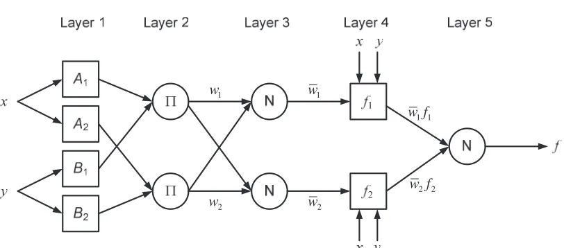
systems to facilitate learning and adaptation [23]. Such framework makes the ANFIS modeling more systematic and less dependent on expert knowledge. In order to present ANFIS architecture, two fuzzy if-then rules based on a first-order Sugeno model are considered:

Rule 1: If (x is A1) and (y is B1) then f1= p x1 +q y1 +r1.

Rule 2: If (x is A2) and (y is B2) then f₂ = p x₂ +q y₂ +r₂.

where x and y are the inputs, fi are the outputs within the fuzzy region specified by the fuzzy

rule, Ai and Bi are the fuzzy sets, { , , }p q r_{i i i} is a set of design parameters that are determined

during the learning process. The ANFIS architecture to implement these rules consists of five layers as shown in Fig. 1. In this architecture, circles indicate fixed nodes and squares indicate adaptive nodes. Nodes within the same layer perform identical functions as detailed below.

Fig. 1 Schematic of ANFIS architecture

2

1

1

( ), 1, 2 ( ), 3, 4 i

i

i A

i B

O x i

O y i

µ µ − = = = = (17)

Theoretically, ( )

i

A x

µ and µB_i( )y can adopt any fuzzy membership function. For example, if the bell functions are chosen then:

2

1

( ) , 1, 2

1 i i A b i i x i x c a

µ

ª_{§ ·} º

−

« »

+ ¨ ¸

«© ¹ »

¬ ¼

(18)

where {ai, bi, ci} are the modifiable parameters governing the shape of the membership

functions. Parameters in this layer are referred to as premise parameters.

Layer 2: The nodes are fixed nodes denoted as Π, indicating that they perform as a simple multiplier. Each node in this layer calculates the firing strengths of each rule via multiplying the incoming signals and sends the product out. The outputs of this layer can be represented as:

2

( )

( ),

1, 2

i i

i i A B

O

=

w

=

µ

x

µ

y

i

=

Layer 3: The nodes are also fixed nodes. They are labeled with N, indicating that they play a normalization role to the firing strengths from the previous layer. The ith node of this layer calculates the ratio of the ith rule’s firing strength to the sum of all rules’ firing strengths:

3

1 2

,

1, 2

i i

i i

i

w

w

O

w

i

w

w

w

=

=

=

=

+

¦

Layer 4: The nodes are adaptive nodes. The output of each node in this layer is simply the

product of the normalized firing strength and a first order polynomial. Thus, the outputs of this layer are given by:

4

( )

i i i i i i i

O =w f =w p x+q y+r (21)

where w_iis the output of layer 3, and {pi, qi, ri} are consequent parameters.

Layer 5: There is only a single fixed node labeled with Σ. This node performs the summation of all incoming signals. Hence, the overall output of the model is given by:

5

, 1, 2

i i i i i i

i i

i

w f

O w f i

w

= = =

¦

¦

¦

Learning algorithm of ANFIS: The task of the learning algorithm for ANFIS architecture is to

tune all the modifiable parameters, namely premise parameters {ai, bi, ci} and consequent

architecture, it can be observed that when the values of premise parameters are fixed, the output of network can be expressed as a linear combination of the consequent parameters:

1 1 2 2

1 1 1 1 1 1 2 2 2 2 2 2

( ) ( ) ( ) ( ) ( ) ( )

f w f w f

w x p w y q w r w x p w y q w r

= +

= + + + + + (23)

The least squares method can be easily used to identify the optimal values of these parameters. When the premise parameters are not fixed, the search space becomes larger and convergence of the training becomes slower. A hybrid algorithm combining the least squares method and the gradient descent method is adopted to solve the problem. The hybrid algorithm is composed of a forward pass and a backward pass. In the forward pass, the least squares method is used to optimize the consequent parameters with the fixed premise parameters. Once the optimal consequent parameters are found, the backward pass commences immediately. In the back pass, the gradient descent method is used to adjust the premise parameters corresponding to the fuzzy sets in the input domain, whilst the consequent parameters remain fixed. This procedure is repeated until either the squared error is less than a specified value or the maximum number of training epoch is encountered.

3. Proposed system

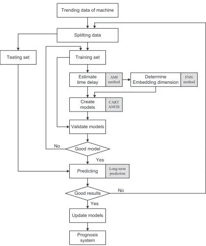
The proposed system for prognosis of machine condition comprises four procedures sequentially as shown in Fig. 2: data acquisition, data splitting, training-validating model, and predicting. The role of each procedure is explained as follows:

Step 1 Data acquisition: this procedure is used to obtain the vibration data from machine condition. It covers a range of data from normal operation to obvious faults of the machine.

Step 2 Data splitting: the trending data attained from previous procedure is split into two parts: training set and testing set. Different data is used for different purposes in the prognosis system. Training set is used for creating the prediction models whilst testing set is utilized to test the trained models.

Step 3 Training-validating: this procedure includes the following sub-procedures: estimating

the time delay and determining the embedding dimension based on AMI and FNN method, respectively; creating the prediction models and validating those models. Validating the prediction models are used for measuring their performance capability.

Step 4 Predicting: multi-step ahead or long-term direct prediction method is used to forecast the future values of machine condition. The predicted results are measured by the error between predicted values and actual values in the testing set. Models and updated data are also carried out in this procedure for the next prediction time.

4. Experiment

The proposed method is applied to a real system to predict the trending data of a low methane compressor which is an important equipment in petrochemical plant.This compressor shown in Fig. 3 is driven by a 440 kW motor, 6600 volt, 2 poles and operating at a speed of 3565 rpm. Other information of the system is summarized in Table 2.

Fig. 3 Low methane compressor: wet screw type. Table 2 Information of the system

The condition monitoring system of this compressor consists of two types: off-line and on-line. In the off-line system, the vibration sensors are installed along axial, vertical, and horizontal directions at the locations of drive-end motor, non drive-end motor, male rotor compressor and suction part of compressor. In the on-line system, acceleration sensors are located at the same places as in the off-line system but only in the horizontal direction.

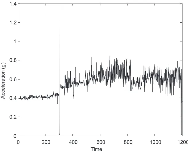
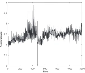
The trending data was recorded from August 2005 to November 2005 which included peak acceleration and envelope acceleration data. The average recording duration was 6 hours during the data acquisition process. This data consists of approximately 1200 data points as shown in

Figs. 4 and 5, and contains information of machine history with respect to time sequence (vibration amplitude). Consequently, it can be classified as time-series data. The proposed method is employed to predict the future condition of vibration amplitude based on the past and current states.

Fig. 4 The entire peak acceleration data of low methane compressor. Fig. 5 The entire envelope acceleration data of low methane compressor.

The machine is in normal condition during the first 300 points of the time sequence. After that time, the condition of the machine suddenly changes. This indicates that there are some faults occurring in the machine. These faults were identified as the damages of main bearings of the compressor (notation Thrust: 7321 BDB) due to insufficient lubrication. Consequently, the surfaces of these bearings were overheated and delaminated [15].

5. Results and discussions

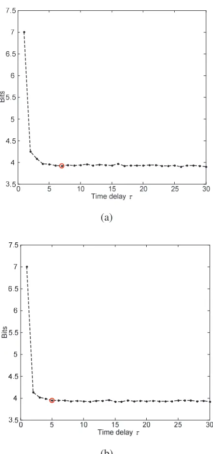
initially calculated according to the method mentioned in section 2.2. Theoretically, the optimal time delay is the value at which the AMI obtains the first local minimum. From Fig. 6, the optimal time delay of peak acceleration training data is found as 7.Similarly, 5 is the optimal time delay value of envelope acceleration training data.

Fig. 6 Time delay estimation. (a) Peak acceleration, (b) Envelope acceleration.

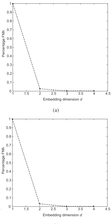
Using FNN method described in section 2.3, the optimal time delay τ is subsequently utilized to determine the embedding dimension d. It is noted that the tolerance level Rtol and threshold

Atol must be initially chosen. In this study, Rtol = 15 and Atol = 2 are used according to [17]. The

relationship between the false nearest neighbor percentage and the embedding dimension for both peak acceleration data and envelope data is shown in Fig. 7. From the figure, the embedding dimension d is chosen as 4 for both data sets where the false nearest neighbor percentage reaches to 0.

Fig. 7 The relationship between FNN percentage and embedding dimension. (a) Peak acceleration, (b) Envelope acceleration.

After calculating the time delay and embedding dimension, the process of generating the prediction models is carried out. Based on the time delay and embedding dimension values, the training data is created as mentioned in section 2.1.3. Using this training data, the CART model and the ANFIS model are established. In case of the CART model, the number of response values for each terminal node in tree growing process is 5 and 10 cross-validations are decided for selecting the best tree in tree pruning. Furthermore, in order to evaluate the predicting performance, the root-mean square error (RMSE) is utilized as following

(

)

N y y RMSE

N

i i i

¦

= 1

2

ˆ

(24) where N, yi, ǔi represent the total number of data points, the actual value, and predicted value

of prediction model in the training data or testing data, respectively.

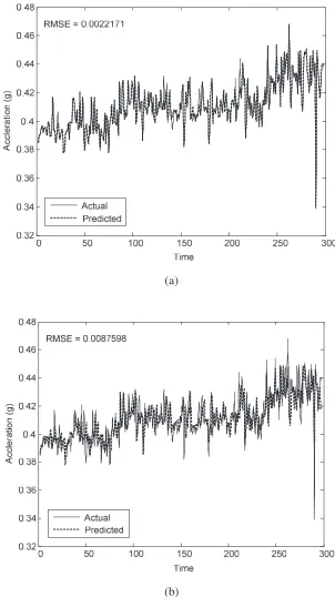
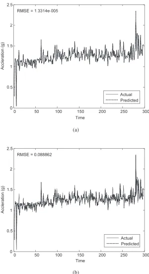
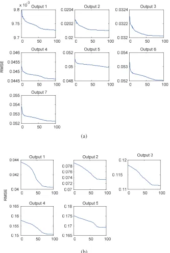
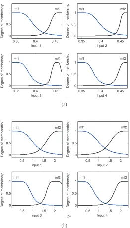
input, a bell shape is chosen for each membership function (MF) and the number of MFs is 2. It means that the region value of each input is divided into two, namely, small and large. In order to evaluate the learning process, the convergence of RMSE is utilized. If the decreasing rate of the RMSE as well as the performance is not significant, the learning process can be terminated. In this study, after executing 100 epochs, all RMSEs of the outputs reach the convergent stage for both the peak acceleration data and envelope acceleration data as shown in Fig. 10. Alternatively, the parameters of MFs, which arepremise parameters and consequent parameters, are automatically adjusted through the learning in order that the outputs of ANFIS model match the actual values in training data. The changes of MF shapes are depicted in Fig. 11. The training and validating results of ANFIS models for both the peak acceleration data and envelope acceleration data are respectively shown in Figs. 8(b) and 9(b). From these figures, the RMSE values are sequentially 0.00876 and 0.08886. These values are higher than those of the CART models. The reason could be that the number of MFs is improperly chosen. For higher accuracy of RMSEs, the MFs can be increased. Nevertheless, this will also increase the computational complexity and take too much training time.

Fig. 8 Training and validating results of peak acceleration data. (a) CART, (b) ANFIS Fig. 9 Training and validating results of envelope acceleration data. (a) CART, (b) ANFIS.

Fig. 10 RMSE convergent curve. (a) Peak acceleration, (b) Envelope acceleration. Fig. 11 The changes of MFs after learning. (a) Peak acceleration, (b) Envelope acceleration.

Figs. 12 and 13 show the predicted results of the CART models and the ANFIS models for peak acceleration and envelope acceleration data.The RMSE values of the CART model and the ANFIS model for those data are summarized in Table 3. Although, the RMSEs of ANFIS models are slightly higher values than those of CART models in both cases of peak acceleration and envelope acceleration data, the predicted results of ANFIS models can keep track with the changes of the operating condition of machine more precisely. This is of crucial importance in industrial application for estimating the time-to-failure of equipments. As mentioned above, the predicted results of ANFIS models can be improved by adjusting the parameters of ANFIS. However, these changes should take into consideration the increase of computational complexity and time-consumption of the training process which may lead to unrealistic application in real life.

Table 3 The RMSEs of CART and ANFIS

5. Conclusion

Machine condition prognosis is extremely essential in foretelling the degradation of operating conditions and trends of fault propagation before they reach the final failure threshold. In this study, multi-step ahead direct prediction for the operating conditions of machine based on data-driven approach has been investigated. The CART models and ANFIS models are validated by its ability to predict future state conditions of a low methane compressor using the peak acceleration and envelope acceleration data. The predicted results of CART models are slightly better than those of ANFIS. Nonetheless, they are incapable of tracking the change of machines’ operating conditions with high accuracy as compared to ANFIS models. The tracking-change capability of operating conditions is of crucial importance in estimating the RUL of industrial equipments. This means that ANFIS has the potential for using as a tool to machine condition prognosis.

References

[1] A.H.C. Tsang, Condition-based maintenance: tools and decision making, Journal of Quality in Maintenance Engineering, 1 (1995) 3–17.

[2] M. Bengtsson, Condition based maintenance system technology – where is development heading, Proceeding of the 17th European Maintenance Congress, 11-13 May (2004), Barcelona, Spain, B-19.580-2004.

[3] M. Abbas, A.A. Ferri, M.E. Orchard, G.J. Vachtsevanos, An intelligent diagnostic/ prognostic framework for automotive electrical systems, Intelligent Vehicles Symposium, 2007 IEEE, 13-15 June (2007), 352–357.

[4] F. Tu, S. Ghoshal, J. Luo, G. Biswas, S. Mahadevan, L. Jaw, K. Navarra, PHM integration with maintenance and inventory management systems, Aerospace Conference, 2007 IEEE, 3-10 March (2007) 1–12.

[5] Y. Li, S. Billington, C. Zhang, T. Kurfess, S. Danyluk, S. Liang, Adaptive prognostics for rolling element bearing condition, Mechanical Systems and Signal Processing 13 (1999) 103–113.

[6] Y. Li, T.R. Kurfess, S.Y. Liang, Stochastic prognostics for rolling element bearings, Mechanical Systems and Signal Processing 14 (2000) 747–762.

[7] M. Watson, C. Byington, D. Edwards, S. Amin, Dynamic modeling and wear-based remaining useful life prediction of high power clutch systems, Tribology Transactions 48 (2005) 208–217.

[8] M. Luo. D. Wang, M. Pham, C.B. Low, J.B. Zhang, D.H. Zhang, Y.Z. Zhao, Model-based fault diagnosis/prognosis for wheeled mobile robots: a review, Industrial Electronics Society ,32nd Annual conference of IEEE, 6-10 Nov. (2005) 2267–2272.

[9] M. Schwabacher, K. Goebel, An survey of artificial intelligence for prognostics, AAAI Fall Symposium on Artificial Intelligence for Prognostics, 9-11 Nov. (2007).

[10]G. Vachtsevanos, P. Wang, Fault prognosis using dynamic wavelet neural networks, AUTOTESTCON Proceedings, IEEE Systems Readiness Technology Conference, 22-23 Aug. (2001) 857–870.

based on self-organizing map and back propagation neural network methods, Mechanical Systems and Signal Processing 21 (2007) 193–207.

[12]W.Q. Wang, M.F. Golnaraghi, F. Ismail, Prognosis of machine health condition using neuro-fuzzy system, Mechanical System and Signal Processing 18 (2004) 813–831.

[13]B. Satish, N.D.R. Sarma, A fuzzy BP approach for diagnosis and prognosis of bearing faults in induction motors, IEEE Power Engineering Society General Meeting 3 (2005) 2291–2294.

[14]E.R. Brown, N.N. McCollom, E. Moore, A. Hess, Prognostics and health management – a data-driven approach to supporting the F-35 Lightning II, Aerospace Conference, 2007 IEEE, 3-10 March (2007) 1–12.

[15]V.T. Tran, B.S. Yang, M.S. Oh, A.C.C. Tan, Machine condition prognosis based on regression trees and one-step-ahead prediction, Mechanical Systems and Signal Processing, in press.

[16]A. Sorjamaa, A. Lendasse, Time series prediction as a problem of missing values: application to ESTSP and NN3 competition benchmarks, European Symposium on Time Series Prediction,7-9 Feb. (2007) 165–174.

[17]M.B. Kennel, R. Brown, H.D.I. Abarbanel, Determining embedding dimension for phase-space reconstruction using a geometrical construction, Physical Review A 45 (1992) 3403– 3411.

[18]L. Cao, Practical method for determining the minimum embedding dimension of a scalar time series, Physica D 110 (1997) 43–50.

[19]D.S. Broomhead, Extracting qualitative dynamics from experimental data, Physica D 20 (1986) 217.

[20]M.T. Rosenstein, J.J. Collins, C.J.D. Luca, Reconstruction expansion as a geometry-based framework for choosing proper delay time, Physica D 73 (1994) 82–89.

[21]A.M. Fraser, H.L. Swinney, Independent coordinates for strange attractors from mutual information, Phys. Rev. A 33 (1986) 1134.

[22]L. Breiman, J.H. Friedman, R.A. Olshen, C.J. Stone, Classification and regression trees, Chapman & Hall (1984).

[23]J.S.R. Jang, 1993, ANFIS: Adaptive-network-based fuzzy inference system, IEEE Trans. System, Man and Cybernetics 23 (1993) 665–685.

[24]A. Sorjamaa, J. Hao, N. Reyhani, Y. Ji, A. Lendasse, Methodology for long-term prediction of time series, Neurocomputing 70 (2007) 2861–2869.

[25]S.E. Shoura, M.E. Sherif, A. Atiya, S. Shaheen, Neural networks in forecasting model: Nile river application, Proceeding of Circuits and Systems, 1998 Midwest Symposium, 9-12 Aug. (1998) 600–603.

[26]Y. Ji, J. Hao, N. Reyhani, A. Lendasse, Direct and recursive prediction of time series using mutual information selection, Lecture Notes in Computer Science 3512 (2005) 1010–1017 [27]J. Jeong, J. C. Gore, B. S. Peterson, Mutual information analysis of the EEG in patients

with Alzheimer’s disease, Clinical Neurophysiology 112 (2001) 827–835.

List of figures

Fig. 1 Schematic of ANFIS architecture.

Fig. 2 Proposed system for machine fault prognosis. Fig. 3 Low methane compressor: wet screw type.

Fig. 4 The entire of peak acceleration data of low methane compressor. Fig. 5 The entire of envelope acceleration data of low methane compressor. Fig. 6 Time delay estimation. (a) Peak acceleration, (b) Envelop acceleration.

Fig. 7 The relationship between FNN percentage and embedding dimension. (a) Peak acceleration, (b) Envelop acceleration.

Fig. 8 Training and validating results of peak acceleration data. (a) CART, (b) ANFIS. Fig. 9 Training and validating results of envelop acceleration data. (a) CART, (b) ANFIS.

Fig. 10 RMSE convergent curve. (a) Peak acceleration, (b) Envelop acceleration.

Fig. 11 The changes of MFs after learning. (a) Peak acceleration, (b) Envelop acceleration. Fig. 12 Predicted results of peak acceleration data. (a) CART, (b) ANFIS.

Fig. 13 Predicted results of envelop acceleration data. (a) CART, (b) ANFIS.

List of tables

Table 1 Training set D for direct prediction strategy.

Table 2 Information of the system.

1 w

2

w

1 1

w f

2 2 w f

2

w

1 w

$0, PHWKRG

)11 PHWKRG

&$57 $1),6

/RQJWHUP

SUHGLFWLRQ

Fig. 3 Low methane compressor: wet screw type.

! "!! #!! $!! %!! &!!! &"!! !

!'" !'# !'$ !'% & &'" &'#

(

)

*

(a)

+

(b)

& &', " "', - -', # #', !

!'& !'" !'-!'# !', !'$ !'. !'% !'/ &

G

(a)

& &', " "', - -', # #',

! !'& !'" !'-!'# !', !'$ !'. !'% !'/ &

G

,

(b)

(a)

(b)

(

)

*

(a)

! ,! &!! &,! "!! ",! -!! !

!', & &', " "',

(

)

*

012!'!%%%$"

(

(b)

(a)

(b)

0.35 0.4 0.45 0 0.5 1 Input 1 D e g re e o f m e m b e rs h ip mf1 mf2

0.35 0.4 0.45

0 0.5 1 Input 2 D e g re e o f m e m b e rs h ip mf1 mf2

0.35 0.4 0.45

0 0.5 1 Input 3 D e g re e o f m e m b e rs h ip mf1 mf2

0.35 0.4 0.45

0 0.5 1 Input 4 D e g re e o f m e m b e rs h ip mf1 mf2 (a) (a)

0.5 1 1.5 2

0 0.5 1 Input 1 D e g re e o f m e m b e rs h ip mf1 mf2

0.5 1 1.5 2

0 0.5 1 Input 2 D e g re e o f m e m b e rs h ip mf1 mf2

0.5 1 1.5 2

0 0.5 1 Input 3 D e g re e o f m e m b e rs h ip mf1 mf2

0.5 1 1.5 2

0 0.5 1 Input 4 D e g re e o f m e m b e rs h ip mf1 mf2 (b) (b)

(a)

! ", ,! ., &!!

3!'" ! !'" !'# !'$ !'% & &'" &'# &'$

(

012!'&.!%

(b)

0 25 50 75 100 0.5

1 1.5 2 2.5 3

Time

A

c

c

e

le

ra

ti

o

n

(

g

)

RMSE = 0.2772

Actual Predicted

(a)

0 25 50 75 100

0.5 1 1.5 2 2.5 3 3.5 4

Time

A

c

c

e

le

ra

ti

o

n

(

g

)

RMSE = 0.29379 Actual

Predicted

(b)

Table 1 Training set D for direct prediction strategy Input X =[X₁,X₂,...,Xd] Output Y =[ ,Y Y1 2,...,Yh]

1 2

[ ,x x ,...,x_d] [xd+1,xd+2,...,xd h+ ]

2 3 1

[ ,x x ,...,x_d+ ] [xd+2,xd+3,...,xd h+ +1]

1 2

[x_{t h d− − +} ,x_{t h d− − +} ,...,x_{t h−} ] [x_{t h− +1},x_{t h− +2},..., ]x_t

Table 2 Information of the system

Electric motor Compressor

Voltage 6600 V Type Wet screw

Power 440 kW

Lobe Male rotor (4 lobes)

Pole 2 Pole Female rotor (6 lobes)

Bearing NDE:#6216, DE:#6216

Bearing Thrust: 7321 BDB

RPM 3565 rpm Radial: Sleeve type

Table 3 The RMSEs of CART and ANFIS

Data type Training Testing

CART ANFIS CART ANFIS