Generalised Design Models For EMS Maglev

University of Huddersfield Repository

Goodall, Roger M.

Generalised Design Models For EMS Maglev

Original Citation

Goodall, Roger M. (2008) Generalised Design Models For EMS Maglev. In: MAGLEV 2008, the  20th International Conference on Magnetically Levitated Systems and Linear Drives, 15th ­ 18th  December 2008, San Diego, USA. (Unpublished) 

This version is available at http://eprints.hud.ac.uk/id/eprint/17942/

The University Repository is a digital collection of the research output of the University, available on Open Access. Copyright and Moral Rights for the items on this site are retained by the individual author and/or other copyright owners. Users may access full items free of charge; copies of full text items generally can be reproduced, displayed or performed and given to third parties in any format or medium for personal research or study, educational or not­for­profit purposes without prior permission or charge, provided:

• The authors, title and full bibliographic details is credited in any copy;

• A hyperlink and/or URL is included for the original metadata page; and

• The content is not changed in any way.

For more information, including our policy and submission procedure, please contact the Repository Team at: [email protected].

Generalised Design Models For EMS Maglev

No. 007

Roger Goodall

ABSTRACT: The paper presents a generic modelling approach for electro-magnetic suspension (EMS) systems which brings together both fundamental principles and specific design factors to provide generalised models that can be adapted for any application. Key system parameters and typical electro-magnetic design factors are used to produce practical models for EMS controller design.

1 INTRODUCTION

Many papers and books have described a variety of models and modelling approaches for use when designing electro-magnetic suspension systems. However, not only are these usually targeted at a particular application [Gottzein and Lange 1975, Shi et al. 2007, Nagurka 1995], but also they adopt a variety of approaches [Sinha 1987, Goodall 1985]. This paper presents a generic modelling approach which brings together both fundamental principles and specific design factors to provide parameterized models that can be adapted and quantified for any application. The paper will concentrate upon linearised models, but implications of the various non-nonlinearities upon the models will be identified and suggestions made regarding the size of parametric changes that should be considered when assessing robustness of the Maglev controller.

Overall the paper will show how some key system parameters and typical design factors can quickly be used to derive practical, quantified models from the generic formulation, targeted particularly towards EMS controller design. Two examples will be introduced to illustrate the modelling approach in practice, one for a larger vehicle suspension magnet, the other for a smaller laboratory levitation system.

2 BASIC EQUATIONS AND NOMENCLATURE

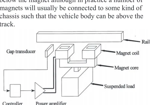
The basic arrangement of a single suspension is shown in Figure 1, here with the suspended load below the magnet although in practice a number of magnets will usually be connected to some kind of chassis such that the vehicle body can be above the track.

Figure 1. Electro-magnetic suspension arrangement

!

F magnet force [N] G airgap [m] Z load position [m] Zt track position [m]

V magnet voltage [V] I magnet current [A] B airgap flux density [T]

Proceedings of MAGLEV 2008 - The 20th International Conference on Magnetically Levitated

"

M suspended mass [kg] N number of turns on coils

A magnet pole area (per pole) [m2] R coil resistance [ȍ]

L magnet leakage inductance [H]

#

g acceleration due to gravity [ms-2] ȝ0 permeability of air [H/m]

$ % &

The equations presented in this sub-section are standard for iron-cored electro-magnets [Mansfield 2007] and are based upon simplifying assumptions that are summarized as each is given.

0 2

2 ) 2 (

P

'

(

)

(1)

This assumes that the flux density B is constant over the pole area and there is no “fringing” of the flux, i.e. spreading out significantly beyond the immediate area of the polefaces.

*

+ ,

-2

0

P

(2)

Here the assumption is that the magnetic circuit is dominated by the reluctance of the two airgaps, which is a reasonable assumption unless the flux density is such that the magnet core is heavily saturated – normally not the case.

Equation (1) and (2) can be combined to give the overall expression for the force (3), although generally it is preferable to use the two separate equations.

2 0 2

2 ) (

*

.

+ ,

/ P

(3)

0 12 3 4 5 6 7 89 : ; < 6 =8> 5 ?

Some published models have current as the input to the magnet, in which case the electrical equations are unnecessary, but in general it is better to include these because voltage is the real input. The voltage has three terms: the ohmic component and two inductive components. The first of the inductive components involves the leakage inductance which relates to the flux leaking between the coils without going through the airgap, the other represents the

mutual inductance which relates to changes in the “useful” magnetic flux in the airgap.

@ A @ B C D @ A @ E

F

G

E

H

(6)

A number of researchers have not distinguished between the absolute movement of the suspended load and the airgap, but properly incorporating the track input is very important when the performance of the maglev suspension system is considered [Goodall 1994]. For this reason there is an important additional equation which is very simple but is sometimes neglected:-

I

I

J K

(7)

For completeness it is useful to include the final equation governing the movement of the suspended mass, i.e. straightforward Newtonian mechanics.

2 2

@ A

I

@

L

M

(8)

Note: the signs are such that increases in Z and ZN

(i.e. upwards movements) cause increasing and decreasing airgap values respectively.

3 MAGNET DESIGN

O PQ L R S T U AVW W VX W Y VA

A number of parameters are inevitably dictated by the specific details of the magnet design and so some consideration is necessary prior to populating the model with numerical values, although it can be shown that these are less profound than might be expected. Note that there will inevitably be dynamic variations in the variables listed in Section 2.1 as the vehicle encounters changing loads and moves along the track – in fact to provide the isolation function of a suspension the airgap must change at higher frequencies in order to absorb the effect of the track irregularities, with corresponding changes in current and flux density. However the main aspects of the magnet design need only consider the nominal values of the variables, indicated using the subscript 0.

Two of the magnet design requirements are a direct consequence of the principal vehicle requirements – the nominal suspension force F0=Mg

and the nominal airgap G0.

The nominal airgap flux density B0 will usually be

but at the same time too low a value will bring an unfavourable increase in the size and weight of the core and coils. From F0 and B0 the pole area can be

straightforwardly determined using equation (1).

The corresponding total excitation is calculated from equation (2), which for 0.7T and an airgap of 10mm works out at a little over 11,000AT – note that to a first approximation, when the pole dimensions are significantly larger than the airgap, the excitation is independent of the pole size. As B0 increases and

portions of the core saturate additional mmf is required to maintain the design level, but this effect is not considered here. Also there is fringing of the magnetic flux which has the effect of reducing the airgap reluctance, thereby increasing the total magnetic flux for a given excitation, but at the same time because of the square law dependence of B upon F the spreading out of the flux reduces the force, and it is not uncommon for these two effects approximately to cancel. The simplified calculation of excitation, i.e. without accounting for the detailed magnetic flux pattern, is usually sufficient for dynamic model development.

O PZ [ \ V] @

U ^

V

S T

The size of the coil is determined by thermal design: strictly this is a question of a combination of the power dissipation in the conductor, the coil surface area and the effectiveness of the cooling, but it is often possible to design on the basis of a specified conductor current density. A practical current density for a copper-coiled magnet is in the region of 1.5-5 A/mm2. However not all the available area will be filled by conductor due to the presence of air gaps, insulation and the coil former so it is also necessary to allow for a "packing factor", a typical value being in the region is 0.6-0.7. The total excitation ampere-turns, divided by the current density and the packing factor, gives the required cross-sectional area of the coil, which is one of the principal determinants of its size.

In order to achieve the defined excitation it is necessary to choose either the number of turns N or the current I0. In practice this decision will be

influenced by the current (or voltage) capability of the magnet power amplifier, although apart from a scaling effect the overall dynamics are largely unaffected by this decision.

Normally the two coils will fill the "slot" between the two poles, meaning that the slot area will be twice this cross-sectional area and a lower current density will therefore increase the size of the core as well as the coil. It is also necessary to decide the aspect ratio

of the winding, although a square cross-section is often a good compromise between minimizing leakage (a wide slot) and not increasing the core size/weight too much. From this it is possible to determine the mean turn length and hence calculate the coil resistance.

Additional influences are the decision between transverse or axial flux magnets (with respect to the direction of travel), rectangular or circular poles, etc. These are however more detailed design considerations, and if available then clearly the information can directly be used to provide model parameters, but the next sub-section will explain an alternative which places less reliance upon detailed design.

O PO _ U ^ VS T ` R W A\ X ^

There is a fundamental trade-off between having a low suspension power (i.e. W/N, or more practically kW/tonne for vehicle magnets) and a good magnet lift/weight ratio. A lower suspension power can only be achieved using a bigger coil which results in a larger, heavier magnet, and vice versa. In practice there are limits for a particular requirement: seeking too low a suspension power will result in an impractical lift/weight ratio, and trying to achieve an ever lighter magnet will eventually be impossible from the thermal design viewpoint.

a b c d ef g h a ijklm n ig o k f p lkb q q n a ijklm n ig o k f p lkb q q n a ijklm n ig o k f p lkb q q n r s s t uvw v uw r x ut y s uz { ux y s ut r w s s t uz z v u{ | uw v uv { ux x s ut y vs s t u| y w uw z x uy { v u| w y u| v v ur r

{ } l~ ~ w r u{ } l~ ~ w w u{ } l~ ~ w

Table 1. Typical magnet design factors (10mm airgap, rectangular poles)

Table 1 gives values for the lift/weight ratio and suspension power derived using normal design methods for different conductor current densities and loads, and illustrates three things:-

1. The design trade-off mentioned in the previous paragraph

2. Lower loads generally result in a less favourable trade-off (assuming the same airgap size)

3. Suspension powers corresponding to reasonable lift/weight ratios are typically in the range from 0.75-2.5 kW/tonne.

It is therefore possible to design to a specified suspension power, which is also a significant system-level performance parameter.

of turns increases the coil resistance by a factor of 4 (half the conductor cross-section area and twice the conductor length), but since the current has halved the I2R loss is unchanged.

4 GENERALISED MODEL FORMULATION

€

PQ

F

V

T U R X V

R

AV\

T

For linearization the variables are re-expressed in terms of small variations about the nominal operating point; hence M ‚ M ƒ „ `

, etc. for the other variables.

0 0 2 0 0 0 0 0 0 0 0 0 0 0 0 0 0 2 2 2 2 … † … ‡ ˆ … † ‰ Š ‹ ˆ † … ‡ ˆ † Œ Š ‹ †  Ž † †  Š  ‹  ‘ ’ w w w w w w P P P (4)

The alternative is to substitute for F = F0 + f, etc.

into the equations and eliminate higher order terms, but this yields the same results for the linearised parameters.

Note that it is also possible directly to linearise equation (3), yielding

0 0 ' ' “ ” • – — ˜ ™ ” • š › w w w w (5)

but when the diagrammatic model is developed it will be seen that the linearised parameters in (4) are more appropriate.

€ PZ L \

@

U

]

^

AX Y W AY X

U

The linearised equations described in the previous section can be best appreciated by showing them in block diagram form, but also it is valuable for control design to have the model in state-space form. Both forms are described, after which the key issues relating to the determination of numerical values for the constants and coefficients will be discussed.

Figure 2 shows the block diagram model, from which the inherently unstable nature of the system is evident from the two negatives in the “physical feedback” from the load position to the flux density and force. The model can be extended for a multi-magnet situation by changing the parts outside the dotted box to represent the rigid (and flexible) dynamics of the vehicle body, with a set of forces from each magnet

impacting on the body system, and a set of airgaps fed back to the magnets from the body system.

1/R+sL

œ  ž Ÿ   ¡ ¢ £ ¤   ¥

66 K_i 66 K_b 1/Ms2

66

Kg

¦ §

¨ © ª

¦ sNA « ¬ ¬ ¬ ­

Figure 2. Block diagram model of single magnet

Conversion into state-space form needs a little care due to the “^C D

” block that represents the induced voltage arising from changes in the airgap flux density, one consequence being that it is necessary for the track input to be represented by its velocity rather than position although this is not a limitation. In fact a variety of formations is possible, depending upon the set of states chosen, but it is useful from a control viewpoint to include the current and the airgap as shown by (8). Note that the output equation is not given because this will depend upon the control approach being used, but it is generally very straightforward to derive.

® ¯ ° ± ¯ ± ¯ ° ¯ ² ³ ´ µ ¶ · ¸ ² ¹ º ¶ ¶ º ¶ ¶ ´ µ ¶ ·

´ µ ¶ ´ µ ¶ · » ¸ ² ¹ » » » ¼ º « « « ¬ ª » » » » » ¼ º « « « « « ¬ ª » » » ¼ º « « « ¬ ª » » » » » » » ¼ º « « « « « « « ¬ ª » » » ¼ º « « « ¬ ª 1 0 0 0 0 1 0 1 0 0 0 (8)

€ PO L \ @ U ] ¼ R X R ½ U AU X ^

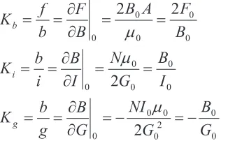
From F0, G0 and B0, equation (4) gives values for

the model parameters Kb and Kg, and of course

equation (1) can be used to calculate the pole area A. Model parameter Ki can then be determined using the

value chosen for I0.

The remaining model parameters are the electrical parameters R and L. As explained in section 3.3, R will depend upon the detailed magnet design, but it is also possible to deduce an approximate value for the resistance without doing a detailed design by assuming a sensible value of specific suspension power, as discussed in Sect 3.3. So, where Ps W/kgf

is the suspension power, this gives I02R/M = Ps, i.e.

The leakage inductance L will depend upon the value of B0, because as the iron in the core becomes

closer to saturation there is more leakage. In the absence of specific design information the leakage inductance can be selected to be a small proportion (e.g. 10%) of the mutual inductance, which, although it is not explicit in the equations, consideration of the block diagram Figure 2 shows that it is given by the expression NAKi.

5 PRINCIPAL APPROXIMATIONS

It will be clear that a number of simplifications have been made in the process of developing the generalized model, and these will result in uncertainties and/or variations in the parameters that need to be accommodated when the suspension controller is being designed and its robustness to parameter variations is being assessed. In fact experience has shown that for general classical control design the model as derived will usually be adequate, but some model-based design approaches are much more susceptible to model uncertainties, and so this section identifies the model parameters that have the more significant variations.

Figure 3. Electro-magnetic non-linearities

Figure 3 illustrates the dominant non-linearities in the electro-magnet:

i) the current-flux characteristic is principally linear but is affected by magnetic saturation in the core and results in a reduced value of Ki compared with

the linearization described in equation (4) – this is indicated by the dotted line. The effect is to increase the changes in excitation compared with the idealized characteristic.

ii) the airgap-flux characteristic is inherently non-linear due to the inverse law, but it is also affected by saturation and again results in a reduced value of Kg. The effect is to reduce the frequency of the

unstable open-loop dynamics and generally to make stabilization a little easier.

iii) the flux-force characteristic is not affected by saturation in the same way and, although there are some effects, the change to Kb is much smaller than

for the other two linearised parameters.

The other factor that will change significantly is the suspended mass M, for which there may be as much as 30% increase as the load varies from empty to full. Associated with the variation in M will be consequential changes in B0 and I0, and the

corresponding changes in Ki, Kb and Kg should be

incorporated, but also the reductions in the first two parameters will become more dominant as increasing B0 brings higher levels of saturation.

6 EXAMPLES

Two examples are used to illustrate the basic

information that is used to provide parameters for the models. The following two sub-sections provide brief descriptions of each and Section 6.3 presents a comparison table.

¾ PQ F \ ¿ À ^¼ U U @ L R S ]U Á Â Ã ^ AU ½

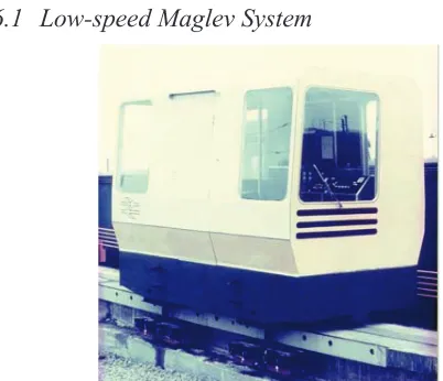
Figure 4. Low-speed 3.2 tonne Maglev vehicle

The vehicle shown in Figure 4 was the experimental version from which the commercialized Birmingham Airport system was derived. It had eight longitudinal flux magnets with rectangular poles, together capable of lifting the full weight of 3,200kg, i.e. 400kg per magnet. Because it was a single stage suspension the airgap was 15mm, relatively large compared with other low-speed Maglev applications of the time, and similarly a relatively high value of B0 was possible because

significant excursions beyond the full load suspension force were not required.

¾ PZ F R Ä \ X R A\ XÃ @ U ½ \ T ^ AX R A\ X

controllers [Hubbard et al. 2008]. It has four longitudinal flux magnets with circular poles, each capable of supporting 50kgf (see Figure 6). As observed earlier, the design of smaller magnets with high flux density is more difficult, and so 0.5 T has been taken for B0, and only a relatively low

lift/weight ratio is achievable.

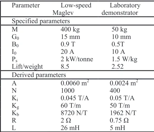
Parameter Low-speed Maglev

Laboratory demonstrator Specified parameters

M 400 kg 50 kg

G0 15 mm 10 mm

B0 0.9 T 0.5T

I0 20 A 10 A

Ps 2 kW/tonne 1.5 W/kg

Lift/weight 8.5 2.52

Derived parameters

A 0.0060 m2 0.0024 m2

N 1000 400

Ki 0.045 T/A 0.05 T/A

Kg 60 T/m 50 T/m

Kb 8720 N/T 1962 N/T

R 2 ȍ 0.75 ȍ

L 26 mH 5 mH

Table 2. Summary of model parameters for example systems

REFERENCES Figure 5. 200kg Maglev demonstrator vehicle

Goodall R.M. “The theory of electromagnetic levitation”, Physics in technology, Vol 16, No5, pp 207-213, September 1985.

Goodall R.M., “Dynamic characteristics in the design of Maglev suspensions” IMechE Proc Pt F, volume 208, pp 33–41, March 1994.

Gottzein E. and Lange B., “Magnetic suspension control system for the MBB high speed train,” Automatica, vol. 11, pp. 271-284, 1975.

Hubbard P., Goodall R.M., Dixon R. and Mapleston M., “Integrated Modular Systems for Maglev Vehicle Control”, Proc 20th International Conference on Magnetically Levitated Systems and Linear Drives (Maglev2008), San Diego, 15-18 December 2008

Figure 6. 50kg magnet

Linder D., “Design and Testing of a low-speed magnetically-levitated vehicle”, Proc. 2nd IEE Conf. Advances in

Magnetic Materials and their Applications, 1976, No 142 pp 96-99.

¾ PO

L

\ @

U

] ¼

R

X

R ½ U

A

U

X

^ ` \ X

U Å R ½ ¼ ]

U ^Ã ^

A

U ½ ^

Table 2 provides an overview of both the design parameters and those for the dynamic model. Both these sets of parameters have been successfully used to provide control system designs for the two applications.

Mansfield A.N., “Electromagnets - Their Design And Construction”, Wexford College Press, 2007

Nagurka M.L., “EMS Maglev vehicle-guideway-controller model”, Proceedings of the American Control Conference, Volume 2, Issue 21-23, pp1167 – 1168, Jun 1995

Shi,J, Wei, Q., Zhao, Y., “Analysis of dynamic response of the high-speed EMS maglev vehicle/guideway coupling system with random irregularity”, Vehicle System Dynamics, Volume 45, Issue 12 , pp 1077 – 1095, December 2007 7 CONCLUSIONS

Sinha P.K., “Electromagnetic Suspension Dynamics and Control, Peter Peregrinus, 1987