A New Robust Multi station Direction Finding Cross Algorithm

2017 International Conference on Computer, Electronics and Communication Engineering (CECE 2017) ISBN: 978-1-60595-476-9

A New Robust Multi-station Direction Finding Cross Algorithm

Hai-ying SUN

1

and Jiang-huai PAN

2,*

1_{Wenjing College, Yantai University, Yantai 264005 China}

2_{Jiangsu Automation Research Institute, Lianyungang 222006 China}

*Corresponding author

Keywords: Direction finding, Passive localization, Modified Singular Value Decomposition(MSVD),

Robust estimation, Localization algorithm.

Abstract. During the multi-station direction finding cross positioning, instable or divergent positioning evaluation result, even invalid situation will occur caused by unreasonable sensor allocation, and analyzes the causes of ill-condition in traditional localization algorithm Therefore, this paper puts forward a kind of stable positioning method based on singular value decomposition modification. The method doesn’t require the station allocation greatly and could consider the resolution and variance assessed by positioning parameter effectively. It realizes effective inhibition to the random observation noise in the observation equation and has better engineering application value. The value simulation result indicates the positioning result is more precise and stable than traditional calculating method.

Introduction

In modern war, passive localization can locate the target radiated by the passive electromagnetic wave. It has a strong concealment and is becoming more and more important in electronic warfare. At present all kinds of electronic warfare systems, electronic reconnaissance equipment generally has a measurement of the target direction, one of the most common parameters of target parameters also can obtain the direction of the station[1,2]_{, multi direction cross positioning method is the earliest and} the technology is relatively mature passive positioning method[3,4]_{. The domestic and foreign} scholars in the multi station cross location precision analysis, optimal station analysis, tracking and elimination of false location has done a lot of work and achieved certain results, but compared with other methods[5,6]_{, the multi station cross location precision of direction finding error influence, in the} localization algorithm[7]_{, optimal station analysis, tracking filter and so there is room for further} improvement[8,9]_.

The multi station DOA algorithm for observability analysis, because the data is less or unreasonable layout of observability resulting in lower case, proposes a modified robust singular value decomposition method based on multi station cross location. The method of the station layout requirements is not high, can effectively combine positioning parameter estimation resolution and variance, to achieve effective suppression of the random observation noise observation equation, which improves the positioning accuracy and stability of estimation of the validity of the simulation results proves that the algorithm.

Multi Station Direction Finding Cross Location Model

i  i  2  2

 1

1

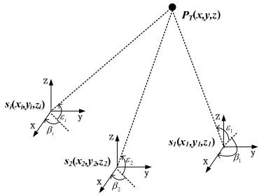
[image:2.612.213.398.67.206.2]



Figure 1. Figure. of multi station direction finding cross location in three-dimensional space.

According to the direction finding value of each sensor, there is the following relation:



 

2



2

tan tan i i i i i i i y y x x z z

x x y y

    _  _   _    _{  }  (1)

Where: i is the sensor number (i=1,…,n), n is the total number of sensors, βi and εi respectively the

ith sensor azimuth and elevation direction finding information,



x y z_i, ,_{i i}



is the sensor in the geographical coordinate system, and



x y z, ,



is the target radiation source in the geographical coordinate system.

The development of equations (1) can be simplified





, 1,...,

i i

A X Z i n (2)

Where: 1 tan 0

tan 0 sin

i i i i A         _   , tan tan sin

i i i

i

i i i i

x y Z x z         _   , x X y z            .

Write all sensor observations(2) in matrix form.

AX Z ₍₃₎

Where: 1 n A A A             , 1 n Z Z Z             .

The least square solution of the formula (3) is:

 

1

ˆ T T

X  A A  A Z (4) Defines the target localization parameter Xas the information matrix:

T

J A A (5)

Ill-Condition Analysis of Target Location Parameter Estimation

caused due to the unreasonable station or the observation noise, due to the influence of random error, the solution is extremely unstable, and the error of localization is very large. From the point of view of numerical solution, formula (3) is ill conditioned, and the accuracy of direct solution formula (4) is very poor. In the common ill conditioned scenes of cross location: when the positions of sensors are closer, that is (x x y y z z 1,  1,  1)(x x y y z z i,  i,  i)_{, the column vectors of matrix A are}

correlated, which leads to the existence of ill-conditioned information matrix J.

In order to effectively evaluate the degree of ill-conditioned, it is necessary to give an index to evaluate it quantitatively. In general, the condition number is evaluated by a number of ill-condition. For the formula(5), small disturbance caused by the estimation of the relative relation of the system error are as follows:

 

cond

X A Z

A

X A Z

  



 

 _  _

  (6)

When the matrix A is nonsingular, the definition of the condition number as follows:

 

cond max _i( ) min _i( )

i i

A 



A



A (7) The coefficient matrix of the value of A is more dispersed, the bigger the cond{A}, the solution vector relative error B is higher. Therefore, to reduce the relative error of the solution vector should be considered to reduce the cond{A}. The condition number is a relative number, and the degree of the minimum characteristic root is the smallest, and the condition number is a measure of the severity of the ill condition. However, there are some relations between the conditions of observation matrix, and it can't be sure that each correlation exists between them. This information has important reference value for us to grasp the mechanism and essence of the ill posed nature, and to determine which of the bias parameters.

Define the condition index:

max _j

j k

k

 



 (8)

k

 define as the matrix of the k condition index, ₁is the maximum eigenvalues, obviously_k 1. The condition index directly reflects the specific system error parameters estimation of influence degree of the measurement noise. If there is high condition index, the column element matrix perturbation, the estimation error of the parameters of the system will cause a considerable change, that there is a relationship between the data column of the observation matrix. Extensive simulation studies show that (Belsley, 1991; Davey, 1959) [12]_{, if the sick is very weak, condition index is less} than 100; pathological condition index is strong, between 100 to 1000; the pathological condition is very serious, the index above 1000.

Robust Estimation Algorithm for Multi Station Direction Finding Cross Location

The LS estimator of formula (3) is the best linear unbiased estimator with the least variance, but in the presence of ill conditioned parameter estimation, the estimation quality of formula (4) becomes worse, and even the results are unreliable, The larger variance makes the formula (4) become a de biased estimator in fact. When the observation equations are ill conditioned, we can be corrected by the rank of the observation matrix to obtain more robust estimation results.

By the Fisher information matrix definition that J is a real symmetric matrix, according to the singular value decomposition theorem for arbitrary symmetric matrix J_{m m} , the existence of orthogonal matrix V_{m m :}

T

Where 0 0 0 S _{ } _

  ,  diag



 

1, ,...,2



r



,  1 2  ... r 0 , i is J eigenvalues;





min ,

r m n . Matrix V _{can be expressed as a column vector of matrix}V 



v v₁, ,...,₂ v_n



. The J Mooer-Penrose generalized inverse is:

1 T

J _VS V ₍₉₎

Where 1



1 1 1



1 , 2 ,..., r ,0,...,0

S diag     The bias estimation of variance:

 

2 2

0 ˆ

D _{b  VS V} T ₍₁₀₎

Written in vector form:

 

2





2

0 1 ˆ

var r i/ i i

b  v 







(11)

From the formula (11) can be seen: if the parameter estimates for the sick, _i 0,so1_i  , and the measurements Z _variance 2

0

 _{will be enlarged, the estimated parameters will be enlarged. In}

this case, the parameter estimation is very unstable, the result is not reliable or even completely wrong. Therefore, we need to modify the



, According to the multi station direction finding cross location algorithm, the eigenvalue distribution of the information matrix is continuous, we used the modified singular value decomposition (MSVD) method to correct the



.

The MSVD method modified _i is out of the above purpose, the value of the _i is modified and not omited, so the number of _i will not be reduced. There are many methods to modify the _i, and the more simple modification is    _i  _{i i},



is more than zero. So the modified _S1

is

1 1

2 2

1 1

,..., r ,0,...,0

r r

S diag













 _  

 _{ } 

  (12)

Written in vector form:





2 1

ˆ r i _, i i

i i i

b_



Z v v

 









(13) The bias estimation of variance:

 

_{2 2}





2

0 1 ˆ

var r _{i i} / _i

i

X_  v   







 (14)

From the formula (13) and formula (14), it can be seen that the proper selection of  can reduce the variance of estimation and increase the stability of estimation.

Simulation Verification

Simulation conditions: two stations simultaneously carry out azimuth and pitch direction finding. The positions of two measuring stations are (10,0,0) and (-10,0,0), and the units are km. Random error of direction finding are

1 2 1

 

   _,

1 2 1

 

   

. The target height is 10km, and the simulation is verified in the range of x:-100 ~ 100km, y:-100 ~ 100km.

accuracy of the improved algorithm is obviously higher than that of the original algorithm, and the cross location accuracy of multi station direction finding is improved better; Figure 6 is an improved GDOP contour map for improved algorithms.

[image:5.612.208.409.114.265.2]

[image:5.612.207.408.295.446.2]

Figure 2. Traditional LS algorithm for locating GDOP grids.

Figure 3. Robust estimation algorithm for locating GDOP grids.

[image:5.612.204.394.478.634.2]

[image:6.612.206.395.68.225.2]

Figure 5. Robust estimation algorithm for locating GDOP contour lines.

Figure 6. Robust estimation algorithm to improve the positioning of GDOP contours.

Conclusion

Aiming at the multi station in DOA Location, location estimation results caused due to sensor layout unreasonable factors such as positioning equation matrix ill condition of instability, divergence and even invalid situation, we analyzes the causes of ill-condition in traditional localization algorithm Therefore, this paper puts forward a kind of stable positioning method based on singular value decomposition modification. The method doesn’t require the station allocation greatly and could consider the resolution and variance assessed by positioning parameter effectively. It realizes effective inhibition to the random observation noise in the observation equation and has better engineering application value. The value simulation result indicates the positioning result is more precise and stable than traditional calculating method.

References

[1]Chen Zhangxin, Wan Qun, Wei Hewen and Yang Wanlin. A Novel Subspace Approach for Hyperbolic Mobile Location. Chinese Journal of Electronics, 2009,Vol 18(3), pp. 569-573.

[2]Hua, Y., W. Wen-Quan and L. Zhong. Observer trajectory optimization of maneuvering target for bearings-only tracking. Proceedings of International Conference of Information Science and Management Engineering (ISME), Xi’an, 2010, pp. 207- 211.

[image:6.612.204.393.253.410.2]

Partial Discharge Source within Power Transformer." Power System Technology 44.1(2005): 86-86.

[4]Zhang, X., Liu, Z., Liu, W., & Xu, Y. (2014). Quasi-vector-cross-product based direction finding algorithm with a Spatially Stretched tripole.Tencon 2013 - 2013 IEEE Region 10 Conference (pp. 1-4). IEEE.

[5]Zhang, Xirui, et al. Quasi-vector-cross-product based direction finding algorithm with a Spatially Stretched tripole. IEEE Xplore 31194(2013): 1-4.

[6]Shen, Xi, et al. A Local Distance Feature Extraction Based Shortwave Direction Finding Cross Location Algorithm. Joint International Mechanical, Electronic and Information Technology Conference 2015.

[7]Chen, T., Han, Q.Q., Liu, L.T., & Lin, J.Q. (2014). Improved wide-band direction finding algorithm based on cross-spectra. XI Tong Gong Cheng Yu Dian Zi Ji Shu/systems Engineering & Electronics, 36(5), 879-883.

[8]Luo, Feng, and X. Yuan. Enhanced "vector-cross-product" direction-finding using a constrained sparse triangular-array. EURASIP Journal on Advances in Signal Processing 2012.1(2012): 115. [9]Yang, Jian, et al. Long baseline direction finding and localization algorithms for noise radiation source. International Conference on Signal Processing IEEE, 2015:52-57.

[10] Yokev, Hanoch, et al. Direction finding and mobile location system for trunked mobile radio systems. US, US 5592180 A. 1997.