Abstract—Green house gas emissions have abraded environmental quality for human existence. Automobile exhaust is a significant contributor globally to green house gases, among other contributors. This research investigates how vehicle fuel consumption can be tabulated from laboratory tests and road tests. The laboratory tests are used to establish mathematical relationships to predict fuel consumption as a function of such drive-cycle parameters as vehicle speed, acceleration and throttle position. Then, these relationships are applied to calculate fuel consumption during real-life road tests. In the future, the drive-cycle parameters contributing to vehicle fuel consumption could be optimized to lower automobile exhaust’s impact on environmental degradation.
Index Terms—Environment, fuel consumption, laboratory testing, new European drive cycle, road testing.
I. INTRODUCTION
Automobile exhaust is a significant contributor to greenhouse gases globally. Out of the global fossil fuel consumption, around 37% is consumed for automobile fuel and industrial purposes [1]. A number of nations have adopted differing greenhouse gas emission standards to lower automobile exhausts. The more stringent standards in this regard have been implemented by Japan and Europe [2]. The various drive cycles associated with differing green house gas emissions standards can be utilized in order to decipher factors that contribute to automobile exhaust and hence environmental degradation [3]. The current research utilizes the European recommended green house gas standard for vehicle exhaust known better as the new European drive cycle (NEDC) for researching factors contributing to automobile exhaust. The central contention is to map the contributing factors and fuel consumption in automobiles to produce a mathematical relationship that can be optimised later. This paper will look into the methods used for and the resulting mathematical relationship between automobile fuel consumption and its contributing factors.
II. NEW EUROPEAN DRIVE CYCLE
A. Mapping the New European Drive Cycle
The NEDC is more aggressive when compared to other drive cycles such as the Japanese cycle or previous European drive cycles [4]. Drive cycles can be segmented into distinct phases that are utilized to emulate real life driving conditions, as shown in Fig. 1. A large number of drive cycles rely on differentiated drive cycle phases such as highway driving, sub-urban driving, motorway driving etc. [5]. In comparison,
Manuscript received September 2, 2014; revised December 16, 2014. The authors are with the University of Huddersfield, UK (e-mail: [email protected], [email protected], [email protected]).
the NEDC is composed in large part only on the urban driving cycle and the extra urban driving cycle. It is felt that most urban drivers experience these driving cycle modes more often than other driving cycle modes such as motorway driving. Moreover, this form of drive cycle allows a more stringent follow up of factors contributin to fuel consumption and hence environmental degradation [6].
B. Urban Driving Cycle
The urban driving cycle is composed of consecutive accelerations, steady speed patches, decelerations as well as idling patches. The contention is to simulate average daily road conditions in any large European city. It needs to be kept in mind that this methodology has been implemented to simulate typical driving conditions based on traffic stops, low speed driving and frequent stops as is typical of any urban driving cycle [7]. However, it would be unrealistic to expect that urban driving alone would suffice for testing purposes, especially for fuel consumption testing purposes, so an extra urban driving mode has also been incorporated for testing. The diagram provided below shows the NEDC graphically in terms of the speed against the testing time.
C. Extra Urban Driving Cycle
[image:1.595.320.529.537.698.2]The EUDC portion of the test, occurring at roughly after 800 seconds of testing is composed roughly half of steady speed driving. The steady speed for testing is maintained between 75 km/hr and 120 km/hr but the testing speed is not pushed any further to accommodate for legal speed restrictions. Moreover, the other half of the EUDC testing cycle is composed of accelerations, decelerations as well as some idling patches [8].
Fig. 1. The new European drive cycle sourced from [3].
III. MATHEMATICAL MODELLING
The NEDC consists of four differentiated cycles of urban driving and one cycle of extra urban (EUDC) driving that have been discussed above. The total resultant drive cycle
Drive Cycle Optimisation for Pollution Reduction
was simulated in laboratory conditions in order to extract quantifiable results for prediction of fuel consumption. Results from laboratory tests were measured and were further used to fit a mathematical function on drive cycle parameters as a means of predicting fuel consumption [3], [6], [8].
A. Mathematical Classification of Phases in NEDC
For the purposes of mathematical modelling the NEDC classifications of urban driving and extra urban driving were decomposed into smaller more quantifiable driving phases. A number of different phases were observed in NEDC components that are listed below:
1) Constant speed driving; 2) Acceleration;
3) Deceleration due to gradient with throttle; 4) Deceleration without gear engagement; 5) Gear change.
These phases may be used to construct any random driving cycle that emulates the different kinds of driving conditions and driving behaviour experienced on both urban and extra urban roads. The fuel consumption of any vehicle driven in these phases depends on several different parameters that are used to describe the driving cycle. An examination of multiple factors was carried out to classify which factors have the greatest effect on fuel consumption. Among the examined parameters, the following ones were observed to exert great influence:
1) Vehicle speed (v); 2) Acceleration (a); 3) Throttle position (p); 4) Gear (G).
The parameters listed above have been used extensively throughout the analysis presented below to propose a mathematical model that can predict fuel consumption (c) in a variety of different driving conditions.
B. Processing of Driving Parameters
Laboratory test runs were used to capture parameter data that was then plotted against the time in order to create a mathematical model. Four different parameters were focused on, namely (i) vehicle speed (in kilometres per hour), (ii) acceleration (in kilometres per hour per second), (iii) throttle position (in percentage opening) and (iv) fuel consumption (in grams per second).The vehicle was sped up and decelerated along with idling stops in order to emulate the NEDC criterion as discussed in preceding sections.
C. Constructing the Relationship between Fuel Consumption and Drive Cycle Parameters
Since the current research is interested in investigating the fuel consumption of the vehicle in relation to the parameters discussed above, the fuel consumption was expressed in terms of these parameters. To make the mathematical model more realistic, the fuel consumption was expressed as different functions of the various parameters in each driving cycle being tested in laboratory conditions. The ordinary least squares regression was utilised to construct mathematical relationships. This required the determination of various constants in such mathematical relationships.
Reference values of each recorded parameter; velocity, acceleration, throttle position and fuel consumption (v0, a0,
p0, and c0) were determined beforehand and these values were
then used in the functions proposed. This allowed the creation of mathematical relationships that could be used independently in a number of situations no matter what units were used to express these parameters. It needs to be kept in mind that the created mathematical relationship would require the insertion of reference values in the same units as the units in which the answer is desirable. The following reference values were used in this study: v0 = 112 km/h (speed limit on motorways in the UK), a0 = 35.316 km/h/s (= 9.81 m/s2), p0 = 100%, and c0 = 0.46 g/s (the average consumption of the studied engine during the NEDC).
D. Constant Speed Phase
First, the case of a constant vehicle speed has been assumed since this provides the simplification of not considering any acceleration terms in the final equation [9]. The relationship between fuel consumption and vehicle speed is assumed to be of a quadratic nature. In this case, the independent variable is settled as the vehicle speed while the dependent variable is settled as the vehicle fuel consumption. Again, any set of units can be utilised as long as the reference parameter assumptions used the same set of units.
0 20 40 60 80 100 120 140 0
0.2 0.4 0.6 0.8 1 1.2 1.4 1.6 1.8 2
Constant speed
Vehicle speed (km/h)
F
u
e
l
c
o
n
s
u
m
p
ti
o
n
(
g
/s
)
[image:2.595.320.537.317.496.2]measured computed
Fig. 2. Fuel consumption in “constant speed” phases in the new European drive cycle.
As shown in Fig. 2, the fuel consumption against vehicle speed can be approximated as a quadratic relationship. It is noticeable that there are data points in the slower speed regions (below 60 kilometers per hour) that are offset from the derived curve. The application of ordinary least squares allows the tabulation of a quadratic curve that is as close as possible to these data points without compromising either the data points or the final curve. The relationship discovered in this fashion can be expressed as:
2
0 0 0
0.3063 0.6532 2.3913
c v v
c v v
(1)
E. Acceleration Phase
assumed with two constants [11].
0 0.5 1 1.5 2 2.5 3 3.5 4 4.5 5 x 10⁻³ 0
0.5 1 1.5 2 2.5
Acceleration
1/(Acceleration*Vehicle speed2) (1/((km/h)3*s))
F
u
e
l
c
o
n
s
u
m
p
ti
o
n
(
g
/s
)
[image:3.595.319.535.51.225.2]measured computed
Fig. 3. Fuel consumption in “acceleration” phases in the new European drive cycle.
The plot in Fig. 3 makes it clear that the relationship between fuel consumption and the parameter derived from acceleration and velocity 1/(av2) emulates power-law like behaviour. It could be argued that plotting fuel consumption against acceleration would produce simpler relationship. However, the presence of vehicle speed in the formula (since acceleration is the rate of change of vehicle speed) tends to complicate matters further and results in a more complex, but a more realistic approximation. A polynomial relationship between fuel consumption and acceleration alone could be produced but it would tend to be cumbersome and prone to errors so the parameter 1/(av2) has been chosen instead after careful consideration. The relationship between fuel consumption and the parameter 1/(av2) can be expressed mathematically with computed constants as follows:
0.3295 2 0 0 2 0
10.1739
a v
c
c
av
(2)F. Decleration Phase
The case of acceleration and deceleration may seem to be connected and simply antipodal to each other at first. However, the case of deceleration is distinguished from acceleration after closer observation. Acceleration only occurs in vehicles when the driver depresses the pedal and causes an increase in the throttle position. In contrast, deceleration of the passenger car may happen under two very different circumstances. First, the vehicle may slow down due to a surface gradient even if the driver depresses the throttle pedal by some amount. Moving the vehicle uphill requires more power; however, without the increase in throttle opening the vehicle speed reduces. In the second scenario, the driver may choose to apply the vehicle’s brakes. The application of brakes would tend to decrease power output to the vehicle’s tyres and lead to deceleration.
In the case of maintained or decreased throttle opening, the fuel consumption is proportional to the product of vehicle speed and throttle position vp. See Fig. 4, when compared with Fig. 3 before makes it abundantly clear that acceleration and deceleration are different phenomenon.
0 500 1000 1500 2000 2500 0
0.5 1 1.5
Deceleration/gradient with throttle
Throttle position*speed (%*(km/h))
F
u
e
l
c
o
n
s
u
m
p
ti
o
n
(
g
/s
)
[image:3.595.65.279.79.261.2]measured computed
Fig. 4. Fuel consumption in “deceleration due to gradient with throttle” phases in the new European drive cycle.
Given the constraints presented above, the relationship between fuel consumption and the parameter vp can be expressed as a linear equation of the form:
0 0 0
0.4675 14.3461
c vp
c v p
(3)
Then, the vehicle may slow down while it is still in gear, but the driver released the throttle pedal. In this case, the fuel is not injected, thus, the fuel consumption drops to zero. Finally, the vehicle may slow down while the gear is in neutral. In this case, the fuel consumption is approximately the same as during idling, which is a special case of the constant speed phase, i.e. when the speed is zero.
G. Gear Change Phase
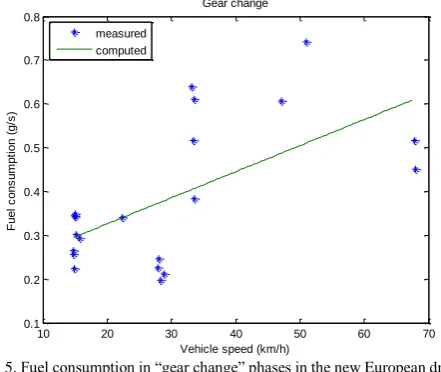
The last phase that is discussed here is the gear change. During gear change, the consumption may vary considerably, but this variation occurs during quite short time intervals (1-3s). Therefore, during this phase the consumption is approximated by a constant that is proportional to the vehicle speed. This relationship was assumed to be linear, although a significant scatter of data can be observed in this phase, as shown in Fig. 5 below.
10 20 30 40 50 60 70
0.1 0.2 0.3 0.4 0.5 0.6 0.7 0.8
Gear change
Vehicle speed (km/h)
F
u
e
l
c
o
n
s
u
m
p
ti
o
n
(
g
/s
)
measured computed
Fig. 5. Fuel consumption in “gear change” phases in the new European drive cycle.
[image:3.595.317.538.558.744.2]0 0 0.4503 1.4494
c v
c v
(4)
H. Compiling the Drive Cycle’s Phases
The functional relationships proposed above can be applied for an arbitrary drive cycle. The drive cycle is divided into short phases, lasting 3-5s each, and the consumption in each of those short phases is determined by the corresponding formula. Then, the total consumption during the whole cycle can be calculated. The application of the obtained relationships to the New European Drive Cycle provides a fuel consumption of 0.460 g/s. The fuel density is 860 g/l; thus, this consumption corresponds to 6.47 l/100 km. The consumption during the same cycle was measured 0.461 g/s (6.49 l/100 km) in laboratory. Thus, the error in the prediction using the proposed formula is 0.3%.
IV. REAL LIFE DRIVING TESTS
Real life driving parameter data was obtained through logging on an actual vehicle, a Golf Mk4 1.9 TDi. The data was acquired using the on board OBDII interface and was later processed through MATLAB. A number of different parameter options were available for logging but four major parameters were logged including:
1) engine speed (rpm); 2) vehicle speed (km/hr); 3) engine load (%);
4) absolute throttle position (%).
0 100 200 300 400 500 600 700
1000 1500 2000
Time(s)
E
n
g
in
e
S
p
e
e
d
(
rp
m
)
Drive Cycle Analysis
0 100 200 300 400 500 600 700
0 20 40
Time(s)
V
e
h
ic
le
S
p
e
e
d
(
k
p
h
)
100 200 300 400 500 600 700
-10 -5 0 5 10
A
c
c
e
le
ra
ti
o
n
(
m
/s
2)
[image:4.595.323.530.326.436.2]Time(s)
Fig. 6. Drive cycle analysis plotted data for the engine speed, vehicle speed and acceleration obtained from Nexiq.
The logged data was utilized in turn to derive other parameters and measurements such as distance, acceleration, fuel consumption etc. The central contention was to compare between the NEDC and real life driving scenarios in order to
derive comparables. A fixed sampling rate was employed to make the logged data more comparable. Logged events and parameters were then classified in terms of vehicle behaviour i.e. cruising, idling, acceleration, deceleration etc. in order to obtain logged runs that could be superimposed onto the NEDC. The gears in use were also tabulated in order to investigate their relationship to parameters. NEDC profiling was also carried out in terms of urban driving and extra urban driving.
Plots were obtained for logged parameters (vehicle speed, acceleration and gradient) as well as for derived parameters (fuel consumption). Parameters were logged and derived as per the NEDC recommendations for the entire test length. The driving cycle parameter analysis for a sample run is plotted in Fig. 6 as a reference.
It must be noted that the vehicle was allowed to soak so that the engine temperature, engine lubricant temperature and coolant temperature achieved their normal values before testing began. This ensured that no variation would occur in measured parameter values as these temperatures changed over the testing time.
TABLEI:SUMMARY OF SALIENT CHARACTERISTICS FOR FIRST TEST Calculated consumption: 0.405 g/s
Total time: 1017.57 S
Total distance: 8.93 Km
Total consumption (mass): 412.22 g
Fuel density: 860 kg/m3 (g/l)
Total consumption (volume): 0.479 L
Consumption: 5.37 l/100 km
From Table I above, the average fuel consumption for the first test was 0.405 g/s that in turn has led to a fuel consumption of approximately 5.37 l/100 km (alternatively 18.62 km/l). Arguably, this fuel consumption figure represents a high value when compared to similar real life driving conditions.
TABLEII:SUMMARY OF SALIENT CHARACTERISTICS FOR SECOND TEST Calculated consumption: 0.38 g/s
Total time: 756.68 S
Total distance: 6.32 Km
Total consumption (mass): 285.65 g
Fuel density: 860 kg/m3 (g/l)
Total consumption (volume): 0.332 L
Consumption: 5.25 l/100 km
From Table II above, the average fuel consumption for the second test was 0.380 g/s that in turn has led to a fuel consumption of approximately 5.25 l/100 km (alternatively 19.05 km/l). Arguably, this fuel consumption figure represents a high value when compared to similar real life driving conditions.
V. CONCLUSION
[image:4.595.54.290.419.707.2] [image:4.595.322.530.543.654.2]above indicates clearly that driving parameters and their outcomes for fuel consumption can be reliably tabulated. Driving tests in laboratory ensure the reliability of the mathematical model derived, which is then applied in real life driving tests. In order to reduce environmental degradation from automobile exhausts, the next logical step would be to optimize the factors contributing to vehicle fuel consumption. It could reasonably be expected that a lowered vehicle fuel consumption would provide for lower automobile exhausts and hence reduced environmental degradation.
REFERENCES
[1] K. Annamalai, “Respiratory quotient (Rq), exhaust gas analyses, CO2
emission and applications in automobile engineering,” Advances in
Automobile Engineering, vol. 2, no. 2, 2013.
[2] P. Ann and A. Sauer, “Comparison of passenger vehicle fuel economy and greenhouse gas emission standards around the world,” Pew Center
on Global Climate Change, pp. 1-33, 2004.
[3] M. Alghadhi, A. Ball et al., “Standard drive cycle recreation from general driving behavior,” in Proc. Computing and Engineering
Annual Researchers Conference, Huddersfield: University of
Huddersfield, 2013, pp. 100-105.
[4] I. M. Berry, “The effects of driving style and vehicle performance on the real-world fuel consumption of U.S. light duty vehicles,” Master's Thesis, Masachusetts Institute of Technology, 2007.
[5] C. Mi, M. M. Abdul, and G. D. Wenzhong, Hybrid Electric
Vehicles:Principles and Applications with Practical Perspectives,
Sussex, U. K.: John Wiley & Sons, 2011.
[6] M. Alghadhi, A. Ball, L. Kollar, R. Mishra, and T. Asim, “Fuel consumption tabulation in laboratory conditions,” in Proc.
International Research Conference on Engineering, Science and
Management, Traders Hotel Dubai, UAE, June 4-5, 2014, pp. 170-180.
[7] National Resarch Council, National Research Council Assessment of
Fuel Economy Technologies for Light-Duty Vehicles, National
Research Council, Washington D. C.: The National Academies Press, 2011.
[8] DEFRA. (2013). Review of Test Procedures EMStec/02/027 Issue 3.
[Online] Available:
http://uk-air.defra.gov.uk/reports/cat15/0408171324_Appendix2Issue 3toPhase2report.pdf
[9] L. Yu, Z. Wang, and Q. Shi, PEMS-Based Approach to Developing and
Evaluating Driving Cycles for Air Quality Assessment, Southwest
Region University, Texas: Transportation Center Texas Transportation Institute, Texas A&M University System, 2010.
[10] W. H. Greene, Econometric Analysis, 5th ed., New Jersey: Prentice Hall, 2002.
[11] M. Alghadhi, A. Ball, L. Kollar, R. Mishra, and T. Asim, “Fuel consumption tabulation in laboratory conditions,” International
Journal of Recent Development in Engineering and Technology, vol. 2,
no. 4, pp. 29-38, 2014.
Mostafa M. Al-Ghadhi was born in Brack, Libya in
1973 and has over 13 years’ working experience in Brega Oil Marketing Company as a maintenance supervisor in mechanical and electrical. He earned his bachelor degree in engineering from the Sebha Higher Institute in 1995, followed by a master degree in energy technology from the University of Salford. Currently he is pursuing a PhD degree from the University of Huddersfield.
![Fig. 1. The new European drive cycle sourced from [3].](https://thumb-us.123doks.com/thumbv2/123dok_us/316106.1032681/1.595.320.529.537.698/fig-new-european-drive-cycle-sourced.webp)