261
FLAW IDENTIFICATION OF METAL MATERIAL IN EDDY
CURRENT TESTING USING NEURAL NETWORK
OPTIMIZED BY PARTICLE SWARM OPTIMIZATION
1ZHAO LIANG, 2Yuxin Mao
1
Lecturer, School of Humanities and Law, Northeastern University, Shenyang, China
2
School of Computer and Information Engineering, Zhejiang Gongshang University, Hangzhou 310018, P.R. China
E-mail: [email protected]
ABSTRACT
As an NDT technology, Eddy current testing is widely used to identify the surface flaw of metal material. However, due to the complex relationship between the test results and the flaw’s shape, the identification is qualitative in most situations. In the paper, a neural network optimized by particle swarm optimization (PSO) is used to quantify the detection result tentatively of the fault on the subsurface of the metal material. Here, PSO is used to optimize the weight value and the threshold value of the BP neural network. According to the experiment, forecasting geometric dimension of the flaws in conductor by PSO-optimized neural network is relatively ideal.
Keywords: Neural Network, PSO, Eddy Current Testing, Surface Fault Identification
1. INTRODUCTION
The detection of the flaw of metal material on their surface or subsurface is critical in many important fields, such as aerospace, military, industrial and so on. Eddy current testing is well suited to inspect the defect on the surface of the metal material. The inspection can be quick, cheap and convenient. Couplant is not required compared to ultrasonic test.
Lift-off effect in the eddy current testing has an important influence on the test result. While the eddy current probe is closed enough to the material which under test, it will limit the testing speed and will wear the probe. In eddy current testing, the impedance value of the test coil is associated with many factors, such as conductivity, thickness, flat of the material, lift off and so on. The relationship between the material characteristics and detect sensor’s output is complex, and it is difficult to describe the relationship in mathematical expression. So the identification of the defect on the surface of the metal material generally speaking is qualitative.
In eddy current flaw detecting research, the lift-off is rarely considered as a variable of quantitative model. However, it has a great influence in the scale and variation of output measures in actual testing. Therefore, this paper will view the lift-off as a variable of the model in
order to build a practicable inverse model for the quantification of eddy current flaw.
2. TRAINING OF ANN PARAMETERS
A. Test specimen and Initial data
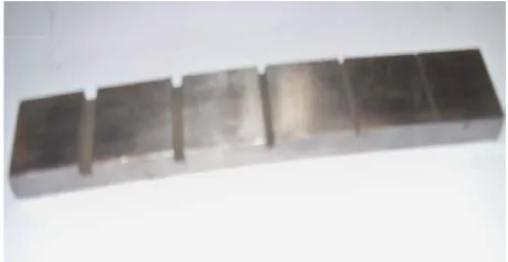
[image:1.612.321.551.538.657.2]The aluminum metal blocks with flaws which are different in depth or width were used in the experiments. And the depth and width of the flaw have different effect on the probe in detecting inductance and resistance. One of the aluminum metal blocks is showed in figure 1.
Figure 1 One Aluminum Block
262
Figure 2 Resistance And Inductance Of The Coil
while the frequency and the scan speed or the shape of the fault is somewhat different in the slope, the figure will be different, but the figure will be similar to the picture showed above.
The impedance value of the test coil carries the physical and geometrical information about the material.
The physical characteristic concludes the conductivity and magnetic permeability. The geometrical characteristic concludes the length, the width, and the depth. Through the figures above, it can be seen easily due to the lift-off, the value of the resistance and inductance is different of the same metal block. The value decays dramatically while the lift-off increases. So the relationship of the flaw’s depth is nonlinear badly to the peak value of the impedance. The lift-off distance must to be considered. The metal flaw identify system is complex, and is difficult to modeling in mathematical technique.
BP neural network can express nonlinear system, it took the system as a black box, based on the input and output data of the system it build network to express the system.
B. Neural network optimized by PSO
Artificial Neural Networks (ANN) can be seen as a system with some intelligence, composed by lots of units parallel connected or series connected together. It has the ability to get knowledge through learning, and then to solve problem, due to self –learning and self-adaptation process. BP network is a multilayer feed-forward neural network, which is used widely in fields such as pattern recognition, image processing, function fitting and so on. One trait of the network is that
the transmission of the signal is forward and the transmission of the error is backward in the network
In BP neural network, the initial weight and threshold values of the neural network is given randomly, so the result will not be the same in different case. Sometimes the result will be satisfactory, but still sometime may be unacceptable. In one word, the result is uncertain, and is related to the initial weight and threshold values badly. In the experiments, a lot of test is taken, the best initial weight and threshold values of the neural network is chosen via the PSO.
PSO is a group intelligence optimization algorithm. It originates from the study of the prey behavior of the birds. The conception of the algorithm is clear, the realization of it is easy, and the parameters which should to be adjusted are little. Every particle in the algorithm represents a potential resolution of the problem. Particles are characteristic by their position, velocity and fitness value. The fitness values are calculated by the fitness function. The fitness value indicates the particle is good or bad. The velocity of the particle determines the direction and the distance of the movement. The velocity of the particle is adjusted dynamic along with the experience of the particle itself and other particles in the group, in order to reach the global optimal solution in the solution space.
A group contains M particles in D dimension space. The status attribute of particle I at the time T is showed below:
Position: t t t t t T i i 1 i 2 i 3 id
( , , , ..., )
x
=x x x
x
[
]
t
id d d d
,
U
,x
∈L
L
is the upper limit andd
U is the
lower limit in search space.
Velocity: t t t t T
i ( i1, i 2, ..., id)
v
=v v
v
t
id min, d, max, d , min
v
∈v
v
v
is the minimum velocity.max
v
is the maximum velocity. The best position of the individual (pbest):t t t t
T
i i1 i 2 id
( ... )
p
=p
+p
+ +p
The best position of the group (gbest):
t t t t T
g1 g 2 gd
g
( ... )
263 Among them 1 d D, 1 i M
Thus the position of the particle I at the time T+1 is renewed according to formula (1-1) and (1-2)
t t
t 1 t t t
1 id 2 id
id id 1 id 2 gd
(
p
) (p
)v
+ =wv
+c
r
−x
+
c
r
−x
(1-1)t 1 t 1 t
id id
v
idx
+ =x
+ + (1-2) w is the inertia weight. r1 and r2 are randomnumbers scatter in the space [0,1], c1 and c2 are
acceleration factors.
The formula of the velocity has three parts. The first part is the former velocity of the particle. The movement of the particle is based on the former state. The second part is the influence of the previous position of the particle itself, and the third part is the influence of the previous position of the group. Therefore, decision-making is based on two important factors, namely, experience of the particle itself and the experience of other particles in the group.
The implementation steps of PSO can be listed as following:
First step:
Initialization. Set the value of Ld, Ud, c1, c2,
vmin, vmax, set the largest iterative times,
convergence precision. Initialize the position and the velocity of the particles randomly.
Second step:
Evaluate every particle. Calculate the fitness value of the particle. If the value is better than the
current pbest , renew the pbest to this position. If the best pbest of all the particals is better than the gbest, renew gbest to the best pbest.
Third step:
Renew the state of the particles. Change the velocity and position of every particles according to the formula (1-1) and (1-2).If vi is larger than
vmax , then set vi as vmax ,if vi is less than vmax ,
then set vi as vmin.
Fourth step:
Judge if terminate condition is meet. Once the iterative times achieve the maximal number set in advance, or the result is fit the convergence precision demand, then stop operation, output the best solution, otherwise turn to the second step.
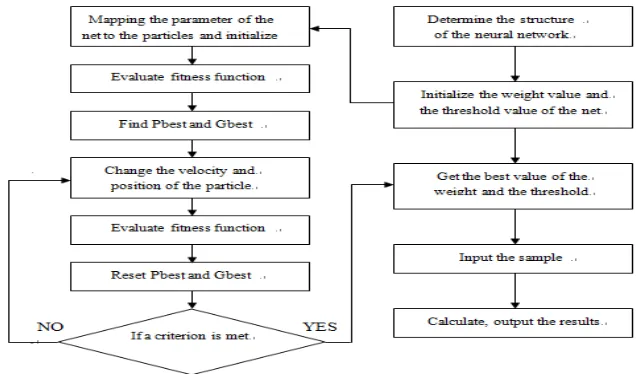
The BP neural network optimized by PSO has three major parts, namely determination of the BP neural network structure, optimization by PSO and prediction of the neural network. The network’s structure is determined by the number of the input and output parameters, once the number of the hidden layer is chosen, the number of the weight and threshold values of the network is determined. Then build the relationship between the particles and the parameters which has to be optimized, in the experiment, the fitness function is the square of the distance between the expectation value of the output and the real value of it.
[image:3.612.137.455.499.686.2]Steps are also shown in Figure 3.
264 C. Implementation and Results
Once got the test curve, reduce the noise first, then take piecewise linear approximation algorithm on the curve. Obtain the length and the slope of each segment. In the test, high frequency and low scan speed is chosen. In the model, the input parameters include length and slope of each fold line, output parameters include liftoff, the width and depth of the rectangular flaw in the test.
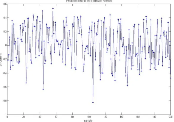
The fitness function of the best particle is showed in figure4. The width of the flaw is easy to calculate, the error between the depth of the flaw calculate by the network and their real value is shown in figure5.
[image:4.612.123.487.229.439.2]The neutral network optimized by PSO takes longer time to build a model than those common ones, but the forecasting precision is obviously higher.
Figure 4 Fitness Function Of The Best Particle
[image:4.612.166.458.469.674.2]265
3. CONCLUSION
The model is built on the premise that some test parameters are determined.
When the material is changed, that is the permeability and the conductivity of the stuff is changed, or the test condition is changed, such as the frequency of the excitation, the speed of the scanning, the net should be retrained. In most cases the material is invariable and the test condition is easy to be fixed. If more than one of these parameters were changed, retrain the net before using. If the time is enough you can build a bigger net to include all these parameters as input or output variables. The net can calculate the depth of the flaw on the surface of the metal, the precision is acceptable, it realize quantitative test in a certain extent. In the experiment while the profile of the flaw is not rectangular, but triangular or semicircle, the impendent curve is similar to that of the rectangular flaw, it is not so easy to distinguish them clearly.
The flaw in the experiment strictly speaking is two dimensional, the next step is to rebuild three dimensional flaw precisely through the neural net which will be more complex, and sort algorithm and feature extraction technique suited in non-linear system should be selected seriously.
REFRENCES:
[1] Y.J. Kenned, R.C. Eberhart, “Particle Swarm
Optimization”, Proceedings of IEEE
International Conference on Neural Networks, 1995, pp. 1942-1948.
[2] R.C. Eberhart, Y.H. Shi, “Particle Swarm Optimization: Developments, Applications and Resources”, Proceedings of the 2011 Congress on Evolutionary Computation, Vol. 1&2, 2001, pp. 81-86.
[3] M. Wrzuszczak, Wrzuszczak, J. Eddy, “Current Flaw Detection with Neural Network Applications”, Measurement, Vol.38, 2005, pp.132-136.