Comparison of Simulation Methods of Ion Atomic Collisions in PIC MC

http://dx.doi.org/10.4236/jamp.2014.213144

Comparison of Simulation Methods of

Ion-Atomic Collisions in PIC-MC

Valeriy Sysun, Alexander Sysun, Vladimir Ignakhin, Viktor Titov, Alexander Tikhomirov Department of Physical Engineering, Petrozavodsk State University, Petrozavodsk, Russia

Email: [email protected], [email protected]

Received 28October 2014; revised 25November 2014; accepted 21December 2014

Copyright © 2014 by authors and Scientific Research Publishing Inc.

This work is licensed under the Creative Commons Attribution International License (CC BY).

http://creativecommons.org/licenses/by/4.0/

Abstract

The main ion-atomic collision treatment methods based on Monte-Carlo simulation are consid-ered and discussed. We have proposed an efficient scheme for simulation of time between colli-sions taking into account cross-section dependence on ion velocity and random generation of ion velocities and scattering angles after collisions. The developed algorithm of simulation of interval between collisions takes into account the change of relative velocity of ion-atom pair as well as the change of cross-section of collision and atomic concentration. At the same time, unlike the widely used “null-collision” method, both the probability of collision and change of particles’ state which determines this probability are taken into consideration for each particle independently in time. The simulation results according to the techniques proposed are found to be close to the theoreti-cal values of ion drift velocities. It is revealed that the “null-collision” method results in exceeding of drift velocity in strong and intermediate fields. At the same time the proposed method of accu-mulation of probability under the same conditions gives values close to theoretical ones. In weak fields calculated values of drift velocity in both methods exceed theoretical values to some small extent.

Keywords

PIC-MC Simulation, Ion-Atomic Collisions, Discharge Plasma

1. Introduction

The drift time of an ion up to the next collision has probabilistic nature: probability of collisions for the time dt doesn’t depend on the previous way and proportional to dt: P

( )

dt = ⋅n u t

( ) ( )

⋅σ u dt, n—concentration of atoms, u t

( )

—relative velocity ion-atom, σ

( )

u —cross-section of collision.

Let us assume by this P′

( )

dt —probability of absence of collision for the time t. Then the probability of collision for dt after non-collision time t, determining decrease of P′ as t increases to dt, is

( )

( )

( ) ( )

( )

dP t′ P t′ n u t σ u dt ρ t dt

− = ⋅ ⋅ ⋅ = ,

where ρ

( )

t is probability density. Equations (1) are the expressions for probability of absence of collision for the time t and for probability density

( )

( ) ( )

( )

( ) ( )

( ) ( )

0 0

exp d ; exp[ d ] .

t t

P t′ = _− nu t σ u t_ ρ t = − ⋅n u t ⋅σ u t n u t⋅ ⋅ ⋅σ u



∫



∫

(1)

Equation (2) is probability of collision since the time t is:

( )

( )

0

d . t

P t =

∫

ρ t′ t′ (2) The following methods of simulation of the interval between collisions are applied.

2. Review of Methods of Simulation of the Interval between Collisions

2.1. Constant Time between Collisions [7]-[9]

Equation (3) is approximation of constant time between collisions

( )

(

)

1

0 n u u const.

τ = ⋅ ⋅σ − = (3)

This approximation is correct at inverse dependence of cross-section on velocity.

In the supposition based on Equation (3)

( )

0 0

1

exp t .

t

ρ

τ τ   = _− _

  Simulation of the random value “τ ” is done

with the help of uniformly distributed at [0,1] random value “rand”. Equation (4) shows the expression for ran-dom value “rand”

( )

0

(

)

0 0

d 1 exp , ln .

rand t t rand

τ _τ

ρ τ τ

τ

−

=

_∫

= − = − (4)

In Equation (4)

(

1−rand

)

is replaced with rand, as it is the random value as well.

2.2. Constant Path Length [5] [6] [9] [10]

Equation (5) is the expression for path length in this case

0 1 const. n λ σ = =

⋅ (5)

Let us replace a variable in Equation (1) dx=u t

( )

⋅dt, then taking into account Equation (5) we will get Equation (6):

( )

0 0 0 0

1 1

exp n xd exp .

λ _λ

ρ λ σ

λ λ λ

    = _− ⋅ _= _− _  



∫

 (6)

For each ion path length is simulated after each collision. Equations (7) are the expressions for ion’s path length

( )

0

(

)

0

(

)

0 0

d 1 exp ; ln 1 or ln .

rand rand rand

λ _λ

ρ λ λ λ λ λ λ

λ   ′ ′

= = − _− _ = − − = −  

The achievement of individual path length by each ion is checked by summing up its ways on each time step

( )

d . i

u t t

λ=

∑

The approximation of constant path length takes into account the change of ion velocity, however the cross- section of collisions is considered to be constant here that can be accepted with some approximation at resonant charge exchange. In [9] a problem of the method considered has been revealed. If the method of constant path length was used, the decrease of average ion energy was observed because of more frequent collisions of fast ions transferring energy to atoms and absence of direct Maxwellian process among charged particles in PIC.

2.3. Simulation of Collision Probability on Each Time Step [1] [3] [11]

For the time interval ∆t relative velocity and cross-section are considered to be constant. Equation (8) is probability of collision for the time ∆t:

( )

( )

(

( )

)

(

)

0

exp d 1 exp .

t

P t n u σ u n u σ u t t n u σ t rand

∆

′ ′

∆ =

_∫

⋅ ⋅ ⋅ − ⋅ ⋅ = − − ⋅ ⋅ ⋅ ∆ = (8)

While each ion is simulated, if rand ≥exp

(

− ⋅ ⋅n u σ

( )

u ⋅ ∆t

)

the collision occurs. Values u and σ cor- respond to the current time point t. This method demands significant increase of computing time that makes it hardly applicable to large ensembles of particles.

2.4. “Null-Collision” Algorithm

This algorithm is considered in details in [2] and actively used [2] [4] [12]. At first, the maximum value of product

(

u⋅σ

)

_max on the whole range of all possible relative ion-atom velocities is determined (or appointed). Upon the value

(

u⋅σ

)

_max the constant conditional collision probability for the time ∆t is calculated. Equa- tion (9) is constant conditional collision probability for the time ∆t

( )

(

)

0 1 exp max

P ∆ = −t _− ⋅ ⋅n u σ ⋅ ∆t_. (9) Then, in case of total number of ions N on each time step,the number of ion is simulated P0N times. For this ion rand is simulated again and the type of collision or the absence of it is defined. Equation (10) is the condi-tion of event that k-type of collision occurs:

( )

1

max

1 1

.

i k i k

i i

i i

uσ rand uσ uσ

= − =

= =

< ⋅ ≤

∑

∑

(10)

At

( )

_max

1

k i i

rand uσ uσ

=

⋅ >

∑

collision doesn’t occur. It compensates for the randomness of choice

( )

uσ _max. Treatment methods of collision probability are combined in the “null-collision” technique. At first, the number of the ion is determined in the ensemble, and then the type of collision or its absence is defined through the change of ion state in time. The number of arithmetic operations

( )

P₀ −1 times is smaller than in the method of determination of collision probability on each time step.

In [12] “null-collision” method is applied to define the collision probability on each time step. At

( )

max

1 exp

rand > − _−n uσ ∆t_ rand is simulated and, if rand⋅

( )

uσ _max >

( )

uσ _i the collision doesn’t occur, and it occurs in the opposite case.

There is a variety of revisions of the “null-collision” algorithm used for simulation of electron-atom collisions when cross-sections are strongly dependent on electrons’ energy. Thus, in the method of constant time between

collisions the time interval is determined by maximum possible value of

(

u σ

)

max τ0

(

n u

( )

σ max

)

1 const

−

⋅ − = ⋅ =

3. Improvement of Methods and Simulation Experiment

3.1. Improvement of Methods of Constant Path Lengths and Time between Collisions—The Method of Accumulation of Probability

It is possible to offer the following method taking into account the change of value σ ⋅n on the ion path. Let us consider expression for density of probability by Equation (1). If according to Equation (11) new variable is in-troduced

( )

0

d d , d ,

t

y n u σ t y t n u σ t

′

′

= ⋅ ⋅ =

_∫

⋅ ⋅ (11)

then we will have ρ

( )

t dt=exp

( )

−y dy for density of probability. Equation (12) is collision probability for the time τ :

( )

( )

( )

( )

( )

0 0

d exp d 1 exp .

y

P t t y y y

τ τ

τ =

_∫

ρ =

_∫

− ′ ′= − _− τ _ (12)

Equations (13) are the expressions if individual ion is simulated:

( )

(

)

1 exp ; i i i ln .

i

y τ rand y n uσ t rand

− _− _= =

∑

∆ = − (13)

Summing up by steps in time lasts up to the reaching of equality in Equation (13). In such a way, this algo-rithm takes into account the change of u as well as the change of σ and n, having approximately the same number of arithmetic operations. At the same time, unlike in the “null-collision” method, both the probability of collision and change of particles’ state which determines this probability are taken into consideration for each particle independently in time. According to the algorithm features it is natural to call this technique “the method of accumulation of probability”.

3.2. Simulation of Energy and Direction of Ion Motion after the Collision

Direction of ion motion after the collision is characterized by taking into account deviation from original direc-tion θ and azimuth angle ϕ. Angle ϕ is equiprobable at symmetrical atoms ϕ=2π⋅rand. In the process of recharge ion velocities after collision are usually taken as equal to atomic ones with Maxwell distribution function [1] [2] [5] [6] [10]. Equation (14) is the expression simulation of θ in this case

cosθ= −1 2rand; 0≤ ≤θ π. (14) At elastic scattering of ion on atom in these works scattering goes only forward. Equation (15) is the formula for θ in this case:

cos 1 ; 0 .

2

rand π

θ= − ≤ ≤θ (15)

Equation (16) is energy after scattering:

2

cos .

ε′ = ⋅ε θ (16) In works [11] [14] at elastic collisions the law of ion-atom interaction is stated. Impact parameter and relative velocity are simulated by randomizer and then depending on the minimal radius of approximation the angles and ion energies are calculated after collision. This method makes simulation process significantly more difficult. At the same time Equations (15), (16) don’t take into account the transfer of energy from atoms to ions that is the most significant at weak fields.

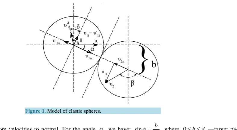
Let us consider Monte-Carlo algorithm of simulation of elastic ion-atom collisions on the model of elastic spheres. In this model in Figure 1 normal and tangential components of ions’ velocity after collision are:

1t 1t

υ′ =υ ; 1

(

)

1 2

2

n n

n

m M M

m M

υ υ υ′ = − +

[image:5.595.143.537.81.298.2]

Figure 1. Model of elastic spheres.

of ion and atom velocities to normal. For the angle α we have:

0

sin b

d

α = , where 0≤ ≤b d0—target pa- rameter, d0—diameter of spheres. We have equal probability of the azimuth angle. Equation (17) is simulation formula for the azimuth angle:

1

2π rand

ϕ= ⋅ . (17)

For the density of probability we have

( )

₂

0

2π d

d 2 d

π

b b

b b b b

d

ρ ′ ⋅ ′= ⋅ ⋅ ′= ′ ′

⋅ , where 0

b b

d

′ = then

2 2

0

2 d

b

rand b b b

′

′ ′ ′

=

_∫

⋅ = . There from one can deduce Equation (18)

2

sinα = =b′ rand . (18)

For strong fields if we ignore atom velocity υ2=0, π 2

θ = −α we get υ1′n=υ2′n=0;

1t 1t 1sin 1cos

υ′ =υ =υ α υ= θ; cosθ= rand2 , it corresponds to Equations (15), (16) taking into account that 1−rand is the same random value like rand.

However, in weak fields an ion can get significant additional velocity from an atom in collisions. Equation (19) is ions’ velocity after collision in this case

( )

2 2 2 2 2

1 1sin 2cos

υ′ =υ α υ+ β, (19)

π 2

θ = − −α δ , cosθ=sin

(

α δ+

)

. Equation (20) is the result for cosθ taking into account that

2 2

1 1

cos tg

sin n

t

υ υ β δ

υ υ α = = :

( )

1

(

_{2 2}

)

1 1 2

cosθ=sinα⋅cosδ +cosα⋅sinδ = υ − ⋅ υ ⋅sin α υ+ ⋅cosβ⋅ 1 sin− α . (20) Let us consider atom υ2 simulation. Equation (21) is the absolute velocity Maxwell distribution function:

( )

3 2 2 2

( )

3 0

4π exp ; d .

2π 2

i

M M

f rand f

KT KT

υ

υ

υ = _ _ ⋅υ _− _ = υ υ

   

∫

(21)

( )

( )

2 2

3 0 4

exp d .

π

t

t t t

rand

υ

υ υ υ

=

_∫

− (22)

The integral can be replaced by an analytic expression, having approximation with accuracy up to 3%. Equa-tion (23) is the approximaEqua-tion for υt

(

)

(

)

0.38

3 2

2

1.30 ln 1 , .

t t

KT rand

M

υ = − − υ =υ (23)

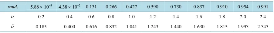
The results of calculations presented in Table 1 reveal the approximation (23) to be close to the exact values. Equation (24) is density of probability of β angles and azimuth angle ϕ2:

(

)

2 2

( )

( )

2 2 2 2 2

sin d d

d 1 sin

, d d ; ; .

2π 2

4π 4π

r S

r r

β β ϕ β

ρ β ϕ β ϕ = = ρ ϕ = ρ β = (24)

It determines cosβ = −1 rand4; ϕ2 =2π⋅rand5.

Angle θ determines the ion deviation from its direction before collision. To determine the ion current in the given direction (along the field) it is necessary to know the angle to this direction (angle θ′ in Figure 2).

Let us have angle θ0 to the axis х up to the collision, θ and ϕ are angles of scattering. Equation (25) is the expression for θ′:

2 2

0 2 0 cos .

θ′ = θ +θ − θ θ⋅ ϕ (25)

0 0 .

θ θ θ θ θ− ≤ ′≤ +

It is here that we need angle ϕ according to Equation (17).

At resonant charge exchange angle θ′ is simulated immediately. Equations (26) are the formulae in this case

1 2

cosθ′= − ⋅1 2 rand, υ υ′= . (26)

3.3. Simulation Experiment

To compare “null-collision” method and method of accumulation of probability the simulation experiment of ion motion in constant electric field E inapproximation to elastic spheres was carried out. The motion with the charge exchange on atoms and elastic interaction was considered separately.

Figure 2. Angles of ion deviation: θ—to the direction up to the

[image:6.595.88.540.668.724.2]

col-lision, θ′—to the direction of the electric field.

Table 1. Comparison of approximated υ_t and exact υ_t values.

rand3 5.88 × 10−3 4.38 × 10−2 0.131 0.266 0.427 0.590 0.730 0.837 0.910 0.954 0.991

t

υ 0.2 0.4 0.6 0.8 1.0 1.2 1.4 1.6 1.8 2.0 2.4

t

The number of ions was taken as equal to 105. Original ion velocities had Maxwell distribution with the tem-perature of atoms by Equations (23) and (24). The interval of time ∆t at integrating motion equations is cho-sen depending on the probability of collision for ∆t according to Equation (9) within P

( )

∆ =t 10 - 0.8.−3 Value

( )

σu _max was accepted in the range of (2 - 20) values, achieved between collisions for the average time. At the same time change

( )

σu _max in the given range practically didn’t influence the average drift velocity. Value σn was taken as constant. Collision process was simulated according to Equations (17)-(26).

Equations (27) are non-dimensional variables accepted:

(

)

; ; ; ln .

i

u u n t t t t x x n y u rand

υ υ′ = ′ =σ ∆ ′= ∆ ′= σ =

∑

′= − (27)

With equations of motion υx′=υx′+a′; x′= +x′ υx′;

2 .

eE

a t n

m σ

′ = ∆

Obtained average drift velocities were compared with theoretical ones [15] [16].

Equations (28) are drift velocities for resonant charge exchange and elastic collision in weak fields when drift velocity is less than thermal velocity:

(

)

(

)

0 1 2 0 1 2

0.332 0.664

and ,

d d

res el

eE eE

mKT n mKT n

υ υ

σ σ

= = (28)

at resonant charge exchange and elastic interaction correspondingly, where σres and σel—cross-sections for resonant charge exchange and elastic collision, respectively. Equations (29) are the corresponding values in strong fields:

1 2 1 2

0.798 and 1.15 .

d d

res el

eE eE

mn mn

υ υ

σ σ

∞ ∞

   

= _{ } = _{ }

    (29)

Equation (30) is the approximation used in intermediate fields:

( )

0

1 2 2

0.252

1 d .

d E d

KT m

υ υ ₌υ _{ +} ⋅ ∞ _

 

  (30)

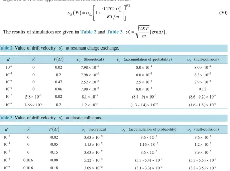
The results of simulation are given in Table 2 and Table 3 t 2

(

)

KT n t m

[image:7.595.91.543.382.717.2]

υ′ = σ ∆ .

Table 2. Value of drift velocity υd′ at resonant charge exchange.

a′ υ′t P( )∆t υd (theoretical) υd (accumulation of probability) υd (null-collision)

10-6 _{0 0.02 7.98 × 10}−4 _{8.0 × 10}−4 _{8.0 × 10}−4

10−4 0 0.2 7.98 × 10−3 8.0 × 10−3 8.3 × 10−3

10−3 0 0.47 2.52 × 10−2 2.5 × 10−2 2.9 × 10−2

10−2 0 0.86 7.98 × 10−2 8.0 × 10−2 0.12

10−6 5.8 × 10−3 0.02 8.1 × 10−5 (8.4 - 9) × 10−5 (8.6 - 9.2) × 10−4

10−4 3.66 × 10−2 0.2 1.2 × 10−3 (1.3 - 1.4) × 10−3 (1.6 - 1.8) × 10−3

Table 3. Value of drift velocity υ_d′ at elastic collisions.

a′ υ′t P( )∆t υd theoretical υd (accumulation of probability) υd (null-collision)

10−5 0 0.02 3.63 × 10−3 3.6 × 10−3 3.6 × 10−3

10−4 0 0.05 1.15 × 10−2 1.16 × 10−2 1.2 × 10−2

10−3 0 0.15 3.63 × 10−2 3.6 × 10−2 3.9 × 10−2

10−4 0.016 0.08 5.22 × 10−3 (5.3 - 5.4) × 10−3 (5.3 - 5.5) × 10−3

It is necessary to mention that computing time in “null-collision” method (in the same conditions) turned out to be 2 - 3 times less than in method of accumulation of probability. However, in case of large P

( )

∆t prob-ability of collision increases more slowly than the velocity achieved for the time between collisions. That results in exceeding of drift velocity in the “null-collision” method. So at P = 0.2; 0.5; 0.8 this exceeding corresponded to approximately 4%; 16%; 40%, respectively.

Method of accumulation of probability in strong and intermediate fields gives values close to theoretical ones. Accuracy is limited only by fluctuations of average velocity increasing when the total number of ions decreases and their temperature goes up. In weak fields calculated values of drift velocity in both methods exceed theo-retical values to some extent (up to 5%). It can be caused by the fact that when Equations (28) are obtained inte-

grated square velocity is accepted as an average relative velocity: 6 d2

KT u

m υ

≈ + .

4. Conclusion

The given effective models of calculating time between collisions by the method of accumulation of probability and ion angle velocities’ simulation after collision on the basis of solid spheres result in ion drift velocities close to theoretical ones and can be applied in the process of simulation of ion motion in heterogeneous plasma with non-constant concentration of atoms and ions and dependence of cross-section on velocity.

Acknowledgements

The work is done by the support of Program of strategic development of Petrozavodsk State University from 2012 to 2016, Ministry of Education of Russian Federation, contract No. 3.757.2014/K.

References

[1] Birdsall, C.K. (1991) Particle-in-Cell Charged-Particle Simulations, plus Monte Carlo Collisions with Neutral Atoms, PIC-MCC. IEEE Transactions on Plasma Science, 19, 65-85. http://dx.doi.org/10.1109/27.106800

[2] Vahedi, V. and Surendra, M. (1995) A Monte Carlo Collision Model for the Particle-in-Cell Method: Applications to Argon and Oxygen Discharges. Computer Physics Communications, 87, 179-198.

http://dx.doi.org/10.1016/0010-4655(94)00171-W

[3] Zobnin, A.V., Nefedov, A.P., Sinel’Shchikov, V.A. and Fortov, V.E. (2000) On the Charge of Dust Particles in a Low-Pressure Gas Discharge Plasma. Journal of Experimental and Theoretical Physics, 91, 483-487.

http://dx.doi.org/10.1134/1.1320081

[4] Cenian, A., Chernukho, A., Bogaerts, A., Gijbels, R. and Leys, C. (2005) Particle-in-Cell Monte Carlo Modeling of Langmuir Probes in an Ar Plasma. Journal of Applied Physics, 97, Article ID: 123310.

http://dx.doi.org/10.1063/1.1938275

[5] Sysun, A.V., Sysun, V.I., Khakhaev, A.D. and Shelestov, A.S. (2008) Charge and Potential of a Dust Grain versus the Intergrain Distance and Establishment of the Latter in a Low-Pressure Plasma. Plasma Physics Reports, 34, 501-507.

http://dx.doi.org/10.1134/S1063780X08060068

[6] Sysun, V.I. and Ignakhin, V.S. (2014) Simulations of the Ion Current to a Probe in Plasma with Allowance for Ioniza-tion and Ion-Neutral Collisions: I. Spherical Probe. Plasma Physics Reports, 40, 101-109.

http://dx.doi.org/10.1134/S1063780X14010097

[7] Kim, H.C., Iza, F., Yang, S.S., Radmilović-Radjenović, M. and Lee, J.K. (2005) Particle and Fluid Simulations of Low-Temperature Plasma Discharges: Benchmarks and Kinetic Effects. Journal of Physics D: Applied Physics, 38, Article ID: R283. http://dx.doi.org/10.1088/0022-3727/38/19/R01

[8] Vaulina, O.S., Repin, A.Y. and Petrov, O.F. (2006) Empirical Approximation for the Ion Current to the Surface of a Dust Grain in a Weakly Ionized Gas-Discharge Plasma. Plasma Physics Reports, 32, 485-488.

http://dx.doi.org/10.1134/S1063780X06060055

[9] Šimek, J. and Hrach, R. (2006) Comparison of Collision Treatment Methods in PIC-MC Plasma Simulation. Czecho-slovak Journal of Physics, 56, B1086-B1090. http://dx.doi.org/10.1007/s10582-006-0331-z

[10] May, P.W., Field, D. and Klemperer, D.F. (1992) Modeling Radio-Frequency Discharges: Effects of Collisions upon Ion and Neutral Particle Energy Distributions. Journal of Applied Physics, 71, 3721-3730.

http://dx.doi.org/10.1063/1.350882

Journal of Physics D: Applied Physics, 28, 324. http://dx.doi.org/10.1088/0022-3727/28/2/015

[12] Boeuf, J.P. and Marode, E. (1982) A Monte Carlo Analysis of an Electron Swarm in a Nonuniform Field: The Cathode Region of a Glow Discharge in Helium. Journal of Physics D: Applied Physics, 15, 2169.

http://dx.doi.org/10.1088/0022-3727/15/11/012

[13] Skullerud, H.R. (1968) The Stochastic Computer Simulation of Ion Motion in a Gas Subjected to a Constant Electric Field. Journal of Physics D: Applied Physics, 1, 1567. http://dx.doi.org/10.1088/0022-3727/1/11/423

[14] Maiorov, S.A. (2009) Ion Drift in a Gas in an External Electric Field. Plasma Physics Reports, 35, 802-812.

http://dx.doi.org/10.1134/S1063780X09090098

[15] McDaniel, E.W. and Mason, E.A. (1973) Mobility and Diffusion of Ions in Gases. Wiley, New York.

[16] Smirnov B.M. (2008) The Sena Effect. Physics-Uspekhi, 51, 291-293.