A New Design of Robust H∞ Load Frequency Controller for Optimal Coordination of Energy Generation in Power System Stability Using LMI Approach

http://dx.doi.org/10.4236/jpee.2015.34021

How to cite this paper: Jaipradidtham, C. and U-thaiwasin, C. (2015) A New Design of Robust H( Load-Frequency Controller for Optimal Coordination of Energy Generation in Power System Stability Using LMI Approach. Journal of Power and Energy Engineering, 3, 146-154. http://dx.doi.org/10.4236/jpee.2015.34021

A New Design of Robust H

∞

_{Load-Frequency}

Controller for Optimal Coordination of

Energy Generation in Power System

Stability Using LMI Approach

Chamni Jaipradidtham

1*

_{, Chatchai U-thaiwasin}

2

1_{Dept. of Electrical Engineering, Faculty of Engineering, Kasem Bundit University, Bangkok, Thailand} 2_{Dept. of Electrical Engineering, Faculty of Engineering, South-East Asia University, Bangkok, Thailand} Email: *_{[email protected]}

Received January 2015

Abstract

This paper presents the problem of robust H∞ load frequency controller design and robust H∞ based approach called advanced frequency control (AFC). The objective is to split the task of ba-lancing frequency deviations introduced by renewable energy source (RES) and load variations according to the capabilities of storage and generators. The problem we address is to design an output feedback controller such that, all admissible parameter uncertainties, the closed-loop sys-tem satisfies not only the prespecified H∞ norm constraint on the transfer function from the dis-turbance input to the system output. The conventional generators mainly balance the low-fre- quency components and load variations while the energy storage devices compensate the high- frequency components. In order to enable the controller design for storage devices located at buses with no generators, a model for the frequency at such a bus is developed. Then, AEC con-trollers are synthesized through decentralized static output feedback to reduce the complexity. The conditions for the existence of desired controllers are derived in terms of a linear matrix in-equality (LMI) algorithm is improved. From the simulation results, the system responses with the proposed controller are the best transient responses.

Keywords

Optimal Coordination, Robust H∞ Controller, Load Frequency Control, LMI Approach

1. Introduction

In power systems, frequency deviations from the nominal value indicate the imbalance between active power supply and consumption. Large unattended frequency deviations could impede the performance of generating units by influencing the performance of their auxiliary electric motor drives and even lead. The control relies on

generating units equipped with local speed droop governors to fast stabilize the frequency while the centralized secondary control is an optimal coordination scheduling task involving economic dispatch and unit commitment programs. In this paper, we focus on the integration of storage into load frequency control (LFC). In this paper incorporates energy limits associated with energy storage and proposes a novel H∞ and structure preserving ap-proach called AFC to integrate energy storage into the framework of frequency control, the decentralized static output feedback and the iterative linear matrix inequality (ILMI) approach are adopted in AFC design.

However, there have recently been only a few reports that combine robust H∞ load frequency controller for power systems with pole-clustering constraints not only to assure in robust stability, but also to improve better transient performance, are derived in terms of LMI in order to construct a desired controller [1].

2. Power System Model

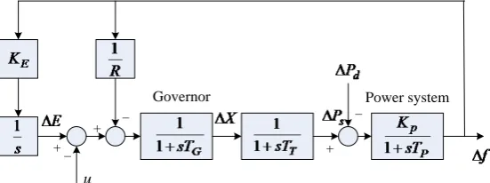
The model of power flow control in Figure 1, considered here. The following simplifying assumptions are made: 1) the power network is represented by a DC power flow model; 2) since the variations in loads within the con-sidered time frame are small compared with the RES disturbances, the loads are assumed to be constant during the small signal analysis, but the same control concept can be applied for load variations and 3) the conventional generators are assumed to be of non-reheat thermal type. In addition, following the general practice in power system analysis.

2.1. Conventional Generator

The considered model of the conventional generator is a fourth order governor-turbine-generator model includ-ing the dynamics of the speed governor and the turbine and is given by [2]

[ ]

0

ref

0 0

0

2 2

0 0 0 0 2

0

1 1 0

0 0

0 1

1 0

0 0 0

N D

N

G e

m m

CH CH

G

G

S k

H HS S

HS

P P

P P

T T

Y Y

T T

ω _ω ω

θ θ

−

 

  _{  − }

 

∆ ∆

   _{    }

 

_∆  _{∆     }

 

 _{= −}  _{+ ∆ +  ∆}

 

 

∆  _{ }∆     

_∆  _{∆     }

 

  ₋  _{    }

 

 

 

 

  



(1)

The parameters and variables in this model are: S_N is power network VA base, S is generator VA base, H is inertia constant based on S,

ω

is rotor speed, ∆ is the deviation from operating point, θ is voltage angle in radians, P_m is mechanical power, P_e is electrical power, k_D is damping factor, T_CH is turbine time con-stant, Y is valve position point, T_G is governor time constant, ω₀ is nominal speed in rad/s. and ref

G

P is con-trol input.

We denote the state space model (1) of the ith conventional generator in a compact form as

, , , , , , ,

G i G i G i G i G i G i e i

x =A x +B u +E P (2) In conventional frequency control, the control input is set to ∆ = −_Gref

(

( ) (

S S R_N

)

)

∆ +ω P_AGC where R is the speed droop coefficient ∆_G of primary control loop and P_AGC is the AGC signal of the secondary control loop.

Governor Power system

u

+ –

– +

+

[image:2.595.159.435.595.698.2]

–

2.2. Energy Storage Device

The storage device consists of the actual storage and the power electronic inverter connecting the device to the grid. The model for the storage captures the relationship between charging/discharging power system, the ener-gy level. The dynamics of the inverter can be modeled using a first order model with time constant T_S captur-ing the response of the inverter to the control signal. The model for the storage device results in the second order model given by

ref

1

0 0

SOC SOC 1 1

0

cap

S

S S

S S

E

P

P P

T T

−

 

 

 

∆ ∆

  _{ } _{   }

= + ∆

 ∆   −  ∆    

  _{ } _{  }

 

 

 (3)

where the parameters and variables are; E_cap is energy capacity in p.u. [3], T_S is inverter time constant,

∆

is the deviation from operating point, SOC is state of charge, P_S is storage power injection and ref

S

P is con-trol input. The power injection ∆P_S can be changed instantaneously in the reduced order model resulting in

[ ][

]

1 ref

SOC 0 ΔSOC _S

cap

P E

⋅  ₋ 

_∆ _{= + ∆ }

 _{  }

 

  _ _ (4)

2.3. Frequency at Load Buses

The challenge which arises in AFC design if the storage is placed at a non-generator bus is the local frequency is not part of the state variables in the traditional power system model.

GG GL

G G G

LG LL

L L L

H H

P H

H H

P

θ θ

θ θ

∆ ∆   ∆

     

= _{ }

_∆  _∆  _∆ 

      (5)

where ∆P_G and ∆P_L are vectors for power injections at generator and non-generator buses; ∆θ_G and ∆θ_L are vectors for voltage angles at generator and non-generator buses; H is the bus admittance matrix.

3. Control Design

3.1. Design of

H

_∞

Controller via LMI Approach

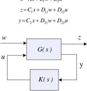
The standard configuration of the H∞ control problem is depicted in Figure 2, where G s

( )

is the transfer

function of the plant, K s

( )

is the transfer function of the controller, ω is the exogenous input including dis-turbances, references and measurement noise, u is the control input, z is the performance vector, we want to mi-nimize to satisfy the control objective and y is the measurement vector [3]-[5]

The corresponding state space model of the standard H∞ control problem in Figure 2 is given as

1 2

x=Ax+B w+B u (6)

1 11 12

z C x= +D w+D u (7)

2 21 22

y C x= +D w+D u (8)

)

s

(

G

)

s

(

K

w

u

z

[image:3.595.222.373.541.698.2]

y

where x is the vector of internal states of G s

( )

. The assumption D₂₂=0 is typically made to simplify calcu-lations without loss of generality. The objective of H∞ control is to find the optimal stabilizing controller

( )

K s that minimizes and the H∞ norm of the transfer functionfrom ω to z, which is defined as the peak of

the maximum singular value control of the complex matrix T_zw

( )

jω over all frequencies ω, that is

( )

sup

(

( )

)

zw zw

T s T j

ω σ ω

∞ 

where T_zw

( )

s is the closed-loop transfer function from ω to z. Consequently, H∞ control gives a guaranteed

bound on the performance vector z for any bounded exogenous input ω, for wind power with given maximal root-mean-square (RMS) variations the resulting control.

The specific design requirements and the focus of the exogenous input signals system, weighting functions are typically assigned to the performance vector and the exogenous input signals, the resulting weighted H∞

control problem becomes [5]

( )

( ) ( ) ( )

min z zw w

K s W s T s W s ∞ (9)

where W_z

( )

s , W_w

( )

s are the matrix valued weighting functions for z and ω, respectively. The matrices allow defining the importance of the individual control.

3.2.

H

_∞

-Based AFC Controller Synthesis

The objectives of AFC design are to minimize the influence of RES variations on frequency deviations and the SOC deviations of the storage devices, and to achieve the frequency separation goal mentioned in Section 1 and the performance vector z in (7) is selected as

T 1, , NG, 1, , NS, m,1, , m N, G, s,1, , S N, S

z= ∆_

ω

 ∆

ω

∆SOC  ∆SOC ∆P  ∆P ∆P  ∆P _ (10) For each of the elements in the performance vector, a frequency dependent weighting function W_{z s( )} as de-fined in (10). These weighting functions are design parameters and reflect the importance of each of the objec-tives along the frequency spectrum of the respective performance element. The weighting functions for the fre-quency deviations ∆ω_i and the SOC deviations, ∆SOCi are chosen to be constant values shown as follows:

( ) (

)

(

)

,

,

10 20π

20π n c

G i n

G i c

s f

W s

m s f

+ =

+ (11)

( )

(

)

(

)

,

,

2π 0.2π

n c

S i n

S i c

s f

W s

m s f

+ =

+ (12)

where f_c is the cut-off frequency in the frequency separation objective, n is the order of the weighting function [5], and m_{G i,} , m_{s i,} are the participation factors of the ith generator, the ith storage device under AFC respec-tively. Hence, where W_{G i,}

( )

s and storage device of W_{S i,}

( )

s with design variables and the weighting function

( )

z

W s in (9) is given by

( )

diag

{

,1, , , G, ,1, , , s, ,1

( )

, , , G

( )

, ,1

( )

, , , s

( )

}

z G G N S S N G G N S S N

W s = η η η η W s W s W s W s (13) where η_G,1 and η_{S i,} are the constant weights values for ∆ω_i and ∆SOCi in the performance vector z.

4. Control System Results

4.1. Output Feedback Controller Design

Theorem 1 The design of system problem, we consider the following norm-bounded uncertain control systems in Figure 1. The uncertainties are described by

( )(

)

1 2

u w

u w

H

A B F

t E E E

H C

∆ ∆ ∆  

 _{= ∆}

 

_{∆ ∗ ∗} 

where ∆C is assumed to be used in practice and * are neglected, our approach for robust H∞ controller with

pole-clustering constraints is proposed [2].

We consider the system and desire to place all closed-loop poles of uncertain systems in D

(

α,r

)

region can be shown as follows:

( )

( )

( )

K K K Ky

x t =A x t +B t (15)

( )

K K

( )

u t =C x t (16) where

( )

nK nK

K

x t ∈ ℜ × is the state of the controller, and A_K, B_K and C_K are matrices with the appropriate dimensions. For a dynamic output feedback controller, we denote its transfer function as follows.

( )

(

)

1

K K K

K s =C sI−A − B (17) Hence, the overall closed-loop system is given by:

( )

( ) ( )

( ) ( )

cl cl cl cl

x t =A ∆ x t +B ∆ w t (18)

( )

cl

( ) ( )

cl

y t =C ∆ x t (19) where

( )

( )

( )

1

(

)

cl cl cl cl x cl cl A B A B

H E E

C C  ∆ ∆  ₌ _{+ ∆}  _{∆ ∗}   _∗      ,

( )

( )

_{( )}

cl K x t x t x t   =     u K cl K K

A B C A

B C A

  =     1 1 2 K H H B H   =    

(

u K

)

E= E E C

0

w cl

F B =   

 

(

0

)

cl

C = C

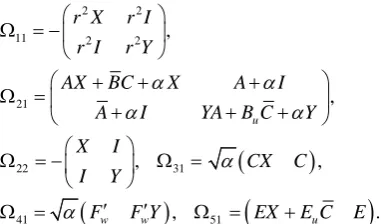
Theorem 2 As for the uncertain linear power system, the desired circular pole region of D

(

α,r

)

and the

H∞ norm bound constraint

γ

>0 on the disturbance rejection are given. The closed-loop system can achieve

the expected performance requirement 1 and 2, if and only if there exist X, Y, A, B, C and a scalar ∈>0

such that [2]

11 21 31 41 51 61

21 22 61

31 2 41 51 61 61 0 0

0 0 0 0 0

0 0 0 0 0 0

0 0 0 0 0

0

0 0 0 0 0 0

0 0 0 0 0 0

0 0 0 0 0 0

0 0 0 0 0 0

w w I I E E I I I I γ α α ′ ′ ′ ′ ′

Ω Ω Ω Ω Ω Ω

 

_{Ω Ω Ω′} 

 

Ω − 

  ′ Ω −   <   − ∈  

_{Ω − ∈} 

 

Ω − ∈

 

 _{Ω′ − ∈} 

 

(20)

where

(

)

(

)

(

)

2 2 11 2 2

21 22 31 41 51 , . , , , , u

w w u

r X r I

r I r Y

AX BC X A I

A I YA B C Y

X I

CX C I Y

F F Y EX E C E

α α

α α

α

α

 

Ω = − 

 

 + + + 

Ω =  

+ + +

 

 

Ω = −_{ } Ω =

 

′ ′

Ω = Ω = +

As a result, a dynamic output feedback controller can be constructed as:

4.2. Problem Analysis

Remark 1 It is obvious that (20) is not an LMI due to the product of a scalar ∈ with variables Y and B, re-spectively. As a result, the LMI software fails to solve (20). However, we are able to achieve difficulty by set-ting ∈ as a prior value and then apply the LMI software. We need to tune ∈ is value until the solver returns a feasible solution.

Remark 2 In LFC problem, when the H∞ constraint is not considered

(

γ → ∞

)

, the problem reduces to

robust LFC controller design with pole-clustering constraints considered as in [2] is reduced to the following LMI: 2 2 1 1 1 1 0 0 0 0 0

0 0 0 0

0 0 0

r P PA PE r P PA PE

A P P H A P P H

EP I EP I

H I H I

α α

α α

− ′ ′  − ′ ′ 

   

− ∈ −

  ₌ _<

 _{− ∈}   ₋ 

   

 _{∈ ′ − ∈}   _{′ −} 

   

(21)

Similarly, when the pole-clustering constraint is absent and the system problem is reduced to the standard of robust H∞ controller design. As a result, (21) is reduced to the following LMI:

Remark 3 It is easy to design the state feedback controller, when all state variables can be available.

1

2

1

0 0 0 0

0 0

0 0

0 0 0

w

w w

w

A P PA PC F PE H

CP I

F r I E

EP E I

H I

′ + ′ ′ ∈

 

 ₋ 

 

 ′ − ′ <

  − ∈    _{∈ ′ − ∈}    (22)

5. Simulation Results

The proposed controllers are applied to the line diagram 8 bus test power system is shown in Figure 3 to illu-strate the performance of the AFC approach. The RES generator is installed at Bus 4 and the energy storage de-vice is placed at Bus 8. The parameter of the test power system, the capacity of the storage dede-vice is 2 MWh with 50 MW maximum power input/output capability, the fact that the energy storage application in frequency regulation is a high power application.The RES variations are within about ±5% around the average value of 600 MW and the RES generator capacity is 800 MW [5].

[image:6.595.202.393.98.210.2]

The Bode magnitude diagram of the transfer functions from the RES disturbance w to the real power output of the three generators and the storage device is depicted in Figure 4. The frequency separation objective in the AFC design is successfully achieved, all the three generators are mainly responsible to balance of the low-fre- quency components of the RES variations below is 0.1 rad/s, the storage device takes of the high-frequency components above 0.1 rad/s, the frequency spectrum up to 3 rad/s.

G

2

1

G

G

10

B

8

B

B

9

2

B

B

4

B

6

_TL

₂₃

_TL

₃₄

B

11

B

12

1

B

5

B

B

7

TL

₂₅

1

F

TL

54

B

14

F

2

13

B

16

B

15

B

17

B

18

B

3

F

3

B

Storage

RES Bus 1

Bus 2 Bus 3

Bus 4

Bus 5 Bus 6

Bus 7

Bus 8

[image:7.595.178.418.90.322.2]

3

[image:7.595.179.420.354.514.2]

Figure 3. Test power system and RES variations.

Figure 4. Real power output in frequency domain.

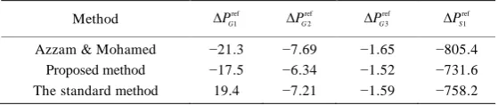
[image:7.595.179.420.538.701.2]

The numerical results of the performance robustness of the proposed controller is superior compared to these methods are shown in Table 1.

The power output deviations of Generator 3 from its operating point are plotted in Figure 6. Similar power output deviation curves are observed for the other two generators. Compared with the base case, the power out-put of the three generators under AFC is smoothed out and high frequency fluctuations in the power outout-put.

6. Conclusions

In this paper, a controller design problem involving both pole clustering constraint and the prespecified H∞

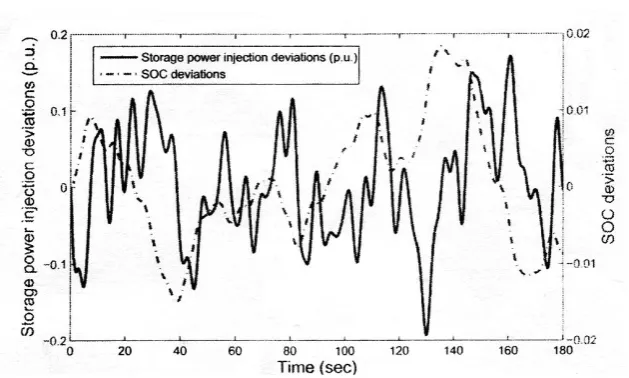
[image:8.595.143.456.297.491.2]

norm constraint for load-frequency control via LMI approach is considered. A proof of concept is given for the AFC design using the 8 bus test system. Under the proposed AFC framework, conventional generators and energy storage devices are coordinated to take the responsibility of power balancing according to the spectrum of the RES variations, high frequency RES variations are balanced by the storage devices, low frequency RES deviations are balanced by the conventional generators reducing the required ramping of the conventional gene-rators. The necessary and sufficient conditions for the existence of a desired controller have proved and the feasible solution to LMI can be used to find a desired controller. In paper comparison with Azzam and Mo-hamed and the standard robust H∞ controller. As can be seen from Figure 7, the power injection deviations

Figure 6. Power output deviations of Generator 2 from its operating point.

[image:8.595.141.456.515.704.2]

[image:9.595.159.437.85.256.2]

Figure 8. Bode magnitude diagram of the transfer function.

Table 1. Comparison of performance robustness: 3 method

Method ref

1 G

P

∆ ref 2 G

P

∆ ref 3 G

P

∆ ref 1 S

P

∆

Azzam & Mohamed Proposed method The standard method

−21.3 −17.5 19.4

−7.69 −6.34 −7.21

−1.65 −1.52 −1.59

−805.4 −731.6 −758.2

and the SOC deviations of the storage device under AFC design. The storage device is sensitive to the high- frequency component of the RES.

The comparison of SOC between AFC and CFC in the frequency domain is plotted as in Figure 8, showing the magnitudes of transfer functions from the RES disturbance (to SOC deviations under AFC and CFC over the entire frequency spectrum. The peak magnitude of the closed loop transfer function from disturbance (to SOC deviations under AFC is approximately −20 dB.

References

[1] Barton, J.P. and Infield, D.G. (2014) Energy Storage and Its Use with Intermittent Renewable Energy. IEEE Transac-tions onEnergy Conversion, 19, 441-448. http://dx.doi.org/10.1109/TEC.2003.822305

[2] Kanchanaharuthai, A. and Nuchkrua, T. (2005) Design of Robust H∞ Load Frequency Control with Pole Clustering Using LMI Approach. EECON-28, 20-21 October 2005.

[3] Vittal, V. (2013) The Impact of Renewable on the Performance and Reliability. PECON Conference, 1, 5-12.

[4] Fiora, R. and Khoi, V. (2009) Large-Scale Frequency Control Solutions Using an H∞ Approach. IEEE Power Energy,

7, 48-57.

[5] Zhu, D. and Hug-Glanzman, G. (2012) Coordination of Storage and Generation in Power System Frequency Control using an Hα Approach. IET Generation, Transmission & Distribution, 7, 1263-1271.

[image:9.595.158.438.301.360.2]