http://dx.doi.org/10.4236/ojop.2015.41002
A New Filled Function with One Parameter
to Solve Global Optimization
Hongwei Lin1, Huirong Li2
1Department of Basic Courses, Jinling Institute of Technology, Nanjing, China
2Department of Mathematic and Computation Application, Shangluo University, Shangluo, China
Email: [email protected], [email protected]
Received 26February 2015; accepted 16March 2015; published 18March 2015
Copyright © 2015 by authors and Scientific Research Publishing Inc.
This work is licensed under the Creative Commons Attribution International License (CC BY). http://creativecommons.org/licenses/by/4.0/
Abstract
In this paper, a new filled function with only one parameter is proposed. The main advantages of the new filled function are that it not only can be analyzed easily, but also can be approximated uniformly by a continuously differentiable function. Thus, a minimizer of the proposed filled func-tion can be obtained easily by using a local optimizafunc-tion algorithm. The obtained minimizer is taken as the initial point to minimize the objective function and a better minimizer will be found. By repeating the above processes, we will find a global minimizer at last. The results of numerical experiments show that the new proposed filled function method is effective.
Keywords
Global Optimization, Filled Function Method, Smoothing Technique, Global Minimize, Local Minimizer
1. Introduction
Global optimization methods have wide applications in many fields, such as engineering, finance, management, decision science and so on. The task of global optimization is to find a solution with the smallest or largest ob-jective function value. In this paper, we mainly discuss the method to find the global minimizer of the obob-jective function. For some problems with only one minimizer, there are many local optimization methods available, for instance, the steepest decent method, the Newton method, the trust region method and so on. However, many problems include multiple local minimizers, and most of the existing methods will not be applicable to these problems.
1) An arbitrary point is taken as an initial point to minimize the objective function by using a local optimi- zation method, and a minimizer of the objective function is obtained.
2) Based on the current minimizer of the objective function, a filled function is designed and a point near the current minimizer is used as an initial point to further minimize the filled function. As a result, a minimizer of the filled function will be found. This minimizer falls into a better region (called basin) of the original objective function.
3) The minimizer of the filled function obtained in 2 is taken as an initial point to minimize the objective function and a better minimizer of the objective function will be found.
4) By repeating steps 2 and 3, the number of the local minimizers will be gradually reduced, and a global minimizer will be found at last.
Although the filled function method is an efficient global optimization method and different filled functions have been proposed, there are some drawbacks for the existing filled functions, such as more than one para- meters to be controlled, being sensitive to the parameters and ill-condition. For example, the filled functions proposed in [1] [2] contain exponent term or logarithm term which will cause ill-condition problem; the filled functions proposed in [3] [4] are non-smooth functions to which the usual classical local optimization methods can not be used; the filled functions proposed in [1] [5] [6] have more than one parameter which is difficult to adjust. To overcome these shortcomings, a new filled function with only one parameter is presented. Although it is not a smooth function, it can be approximated uniformly by a continuously differentiable function. Thus its minimizer can be easily obtained. Based on this new filled function, a new filled function method is proposed.
The remainder of this paper is organized as follows. Related concepts of the filled function method are given in Section 2. In Section 3, a new filled function is proposed and its properties are analyzed. Furthermore, an ap- proximate function of the proposed filled function is given. Finally, the method for avoiding numerical difficulty is presented. In Section 4, a new filled function method is proposed and the numerical experiments on several test problems are made. Finally, some concluding remarks are drawn in Section 5.
2. The Related Concepts
Consider the following global optimization problem with a box constraint:
( )
min( )
x
P f x
∈Ω
where f x
( )
is a twice continuously differentiable function on Rn and[
]
1,
n
n i i i
l u R
=
Ω =
∏
⊂ . Generally, weassume that f x
( )
has only a finite number of minimizers and the set of the minimizers is denoted as{
i 1, 2, ,}
Lm= x i∗ = I in Ω (I is the number of minimizers of f x
( )
). Some useful concepts and notations are introduced as follows:1
x∗: A local minimizer of f x
( )
on Ω found so far; 1S : Set S1
{
x f x( )
f x( )
1 ,x \{ }
x1}
∗ ∗
= ≥ ∈ Ω ;
2
S : Set S2
{
x int f x( )
f x( )
1}
∗= ∈ Ω < ;
m: A constant satisfying
{ }
( ) ( )
( ) ( )
, 1,2, , , min
i j
i j
i j I f x f x
m ∗ ∗ f x∗ f x∗
∈ ≠
= −
;
M : A constant satisfying , max
x y
M x y
∈Ω
= − .
Assumption. All of the local minimizers of f x
( )
fall into the interior of Ω.Definition 1 The basin [7] of f x at an isolated minimizer
( )
x1∗ is a connected domain B x( )
1∗
which contains x1
∗
, and in which the steepest descent sequences of f x starting from any point in
( )
B x( )
1∗ con- verge to x1∗
, while the minimization sequences of f x starting from any point outside of
( )
B x( )
1∗ doesn’t converge to x1∗
. Correspondingly, if x1 ∗
is an isolated maximizer of f x
( )
, the basin of −f x( )
at x1 ∗is defined as the hill of f x at
( )
x1∗.It is obvious that if x B x
( )
1∗
∈ , then f x
( )
f x( )
1∗
> . If there is another minimizer x2 ∗
of f x
( )
and( )
2f x∗ < or f x
( )
2∗
≥ , then the basin B x
( )
2∗
of f x
( )
at x2 ∗is said to be lower (or higher) than B x
( )
1∗
( )
f x at x1 ∗ .
The first concept of the filled function was introduced by Ge [1] [2]. Since the concept of the filled function was introduced, different filled functions are given (e.g., [8] [9]). A new concept of the filled function was presented which is easier to understand in [8]. It can be described as follows:
The first concept of the filled function was introduced in [1].
Definition 2A function FF x is said to be a filled function of
( )
f x at( )
x1 ∗, if it satisfies the following properties:
1) x1 ∗
is a strict local maximizer of FF x
( )
over Ω; 2) FF x( )
has no stationary point in the set S1\{ }
x1∗ ;3) if the set S is not empty2 , then there exists a point x′∈S2 such that x′ is a local minimizer of FF x
( )
. Based on definition 2, we present a new filled function with only one parameter in Section 3.3. A New Filled Function and Its Properties
Assume that a local minimizer x1 ∗
of f x
( )
has been found so far. Consider the following function for pro- blem (P):(
)
(
{
( )
( )
}
)
21 1 1
, , max , 0
FF x x A∗ = − +A f x∗ −f x × −x x∗ (1)
where A is a parameter.
The following theorems will show that the formula (1) is a filled function which satisfies definition 2. Theorem 1 Suppose x1
∗
is a local minimizer of f x and
( )
FF x x A(
, 1∗,)
is defined by (1), then x1 ∗is a strict local maximizer of FF x x A
(
, 1,)
∗
for all A>0. Proof. Since x1
∗
is a local minimizer of f x
( )
, there exists a neighborhood N x(
1,δ)
int∗ ⊂ Ω
of x1 ∗ , 0
δ > such that f x
( )
f x( )
1∗
≥ for all x N x
(
1,δ)
∗
∈ . For all x N x
(
1,δ)
∗
∈ , x x1 ∗
≠ , one has
(
)
2(
)
1 1 1 1
, , 0 , ,
FF x x A∗ = − × −A x x∗ < =FF x x A∗ ∗ (2)
Thus, x1 ∗
is a strict local maximizer of FF x x A
(
, 1∗,)
. □Theorem 2 Suppose x1 ∗
is a local minimizer of f x
( )
, x is a point in set S1, then x is not a stationarypoint of FF x x A
(
, 1,)
∗
for all A>0.
Proof. Due to x∈S1, one has f x
( )
f x( )
1∗
≥ and x x1
∗ ≠ , so
(
)
2(
)
(
)
1 1 1 1
, , , , , 2 0
FF x x A∗ = − × −A x x∗ ∇FF x x A∗ = − A× −x x∗ ≠
Namely x is not a stationary point of FF x x A
(
, 1,)
∗ . □
Theorem 3 Suppose x1 ∗
is a local minimizer of f x but not a global minimizer of
( )
f x( )
, which means2
S is not empty, then there exists a point x′∈S2 such that x′ is a local minimizer of FF x x A
(
, 1,)
∗
when
0< <A m. Proof. Since x1
∗
is a local minimizer of f x
( )
, and x1 ∗is not a global minimizer of f x
( )
, there exists another local minimizer x2∗
of f x
( )
such that f x( ) ( )
2∗ < f x1∗ .By the definition of m and continuity of f x
( )
, there exists a point x in rectangular area x x1, 2∗ ∗
, such that
( )
1( )
f x∗ − f x =A (3)
So
(
1, 1,)
(
, 1,)
0FF x x A∗ ∗ =FF x x A∗ = (4)
By x1 ∗
is a local minimizer of f x
( )
, there exists a point x B x( )
1 x x1, 2∗ ∗ ∗
∈ ∩
such that
(
, 1,)
0Then, there exists a point 1, 2
{
n min{
1 , 2}
i max{
1 , 2}
}
inti i i i
x′∈x x∗ ∗= x∈R x∗ x∗ ≤x ≤ x∗ x∗ ⊂ Ω which is a
minimizer of FF x x A
(
, 1,)
∗
.
Furthermore, by the Theorem 2, one has f x
( )
f x( )
1∗
′ < . Consequently, Theorem 3 is true. □ From Theorem 1, 2 and 3, we know that if there is a better local minimizer x2
∗
of f x
( )
than x1 ∗, then there exists a point x′ which is minimizer of FF x x A
(
, 1,)
∗
. It falls into a lower basin. These mean that if one minimizes f x
( )
with initial point x′, a better minimizer of f x( )
will be found.We can find that if x1 ∗
is not a global minimizer of the objective function, then FF x x A
(
, 1,)
∗
is non-diff- erentiable at some point in Ω. Gradient-based algorithms for local optimization cannot be used to obtain the minimizer of FF x x A
(
, 1,)
∗
. A smoothing technique [10] to approximate FF x x A
(
, 1,)
∗
is employed here as follows.
Let
( )
(
(
(
( )
( )
)
)
)
21 1
1
ln 1 exp
p
FF x A p f x f x x x
p
∗ ∗
= − + + × − × −
(5)
where p is a positive parameter. It is obvious that FFp
( )
x is a differentiable. Further, because( )
(
)
(
(
(
( )
( )
)
)
)
{
( )
( )
}
( )
( )
{
}
(
)
(
)
{
( )
( )
}
21 1 1 1
2
1 1 1
2 1 1
, , ln 1 exp max 0,
1
ln 2exp max 0, max 0,
ln2
p
FF x FF x x A p f x f x f x f x x x
p
p f x f x f x f x x x
p x x p ∗ ∗ ∗ ∗ ∗ ∗ ∗ ∗ − = + × − − − × − ≤ − − − × − = − and
( )
(
)
(
(
(
( )
( )
)
)
)
{
( )
( )
}
( )
( )
{
}
(
)
(
)
{
( )
( )
}
21 1 1 1
2
1 1 1
1
, , ln 1 exp max 0,
1
ln exp max 0, max 0,
0
p
FF x FF x x A p f x f x f x f x x x
p
p f x f x f x f x x x
p ∗ ∗ ∗ ∗ ∗ ∗ ∗ − = + × − − − × − ≥ − − − × − =
we have that the inequality
( )
(
)
22
1 1
ln2 ln2
0 FFp x FF x x A, , x x M
p p
∗ ∗
≤ − ≤ − ≤ (6)
holds. From above discussion, we can see that FFp
( )
x uniformly converges to FF x x A(
, 1,)
∗
as p tends to infinity. Therefore, by selecting a sufficiently large p, the minimization of FF x x A
(
, 1∗,)
can be replaced by( )
min p
x∈ΩFF x (7)
In order to obtain a more precise minimizer of FF x x A
(
, 1,)
∗
by solving FFp
( )
x , p in FFp( )
x shouldbe large enough. However, if the value of p is too large, it will cause the overflow of the function values
( )
pFF x . To prevent the occurrence of this situation, a shrinkage factor r is introduced to FFp
( )
x as follows.First of all, it is necessary to estimate max
( )
min( )
x x
U f x f x
∈Ω ∈Ω
= − and give a fixed and sufficiently large p
(e.g., take it as p=103M2) which guarantees that the FFp
( )
x accurately approximates to FF x x A(
, 1,)
∗
.
Then, in order to prevent the difficulty of numerical computation, a large 10
pU
r= can be taken. Finally,
( )
p( )
( )
1( )
2 1 ln 1 expp
f x f x
r
FF x A p x x
p r
∗
∗
−
= − + + × × −
(8)
By doing so, the existing shortcomings can be overcome.
4. A New Filled Function Algorithm and Numerical Experiments
4.1. A New Filled Function Algorithm
Based on the theorems and discussions in the previous section, a new filled function algorithm for finding a global minimizer of f x
( )
will be proposed, and then some explanations on the algorithm will be given. The details are as follows.Step 1 (Initialization). Choose the initial values
(
A= A0)
(e.g., A0=1), a shrinkage factor 0< <ρ 1 (e.g., 0.1ρ = ), a lower bound of A (denote it as Lba), sufficiently large p and r. Some directions di, 1, 2,i= , 2n are also given in advance, where di=
(
0,, 1 ,∗ i, 0)
T, i=1, 2,,n and di = −di n− , i= +n 1,, 2n, n isthe dimension of the optimization problems. Set k: 1= .
Step 2 Minimize f x
( )
starting from an initial point xk∈ Ω and obtain a minimizer xk∗
of f x
( )
. Step 3 Construct( )
( )
1( )
2 1 ln 1 expp
f x f x
r
FF x A p x x
p r
∗
∗
−
= − + + × × −
Set i=1.
Step 4 If i≤2n, then set x xk δdi
∗
= + and go to Step 5; otherwise, go to Step 6.
Step 5 Use x as an initial point for minimization of FFp
( )
x , if the minimization sequences of FFp( )
xgo out of Ω, set i= +i 1 and go back to Step 4; Otherwise, a minimizer x′ of FFp
( )
x will be found inΩ and set xk =x′, A=A0, k= +k 1 and go back to Step 2. Step 6 If A≤Lba, the algorithm stops and xk
∗
is taken as the global minimizer of f x
( )
; Otherwise, decrease A by setting A:= ×ρ A, go to Step 3;Before we go to the experiments, we have to give some explanations on the above filled function algorithm. 1) In minimization of f x
( )
and FFp( )
x , we need to select a local optimization method first. In the pro-posed algorithm, the trust region method is employed.
2) In Step 4, the smaller δ is needed to select accurately, in our algorithm, the δ is selected to guarantee
( )
p
FF x
∇ is greater than a threshold (e.g., take the threshold as 10−3).
3) Step 5 means that if a local minimizer x′ of FFp
( )
x is found in Ω and with f x( )
f x( )
k∗
′ < , then a better local minimizer of f x
( )
will be obtained by using x′ as the initial point to minimize f x( )
.4.2. Numerical Experiment
In this section, the proposed algorithm is tested on some benchmark problems taken from some literatures. Problem 1. (Two-dimensional function)
( )
(
)
2(
)
22 2 1 2 1
1 2
min 1 2 sin 4π 0.5sin 2π ,
. . 0 10, 10 0
f x x c x x x x
s t x x
= − + − + −
≤ ≤ − ≤ ≤
where c=0.2, 0.5, 0.05. The global minimum solution satisfies f x
( )
∗ =0 for all c. Problem 2. (Three-hump back camel function)( )
2 4 6 21 1 1 1 2 2
1 2
1
min 2 1.05 ,
6
. . 3 3, 3 3
f x x x x x x x
s t x x
= − + − +
− ≤ ≤ − ≤ ≤
Problem 3. (Six-hump back camel function)
( )
2 4 6 2 41 1 1 1 2 2 2
1 2
1
min 4 2.1 4 4 ,
3
. . 3 3, 3 3
f x x x x x x x x
s t x x
= − + − − +
− ≤ ≤ − ≤ ≤
The global minimum solution is x∗= −
(
0.0898, 0.7127−)
T or x∗=(
0.0898, 0.7127)
T, and( )
1.0316f x∗ = − .
Problem 4. (Treccani function)
( )
4 3 2 21 1 1 2
1 2
min 4 4 ,
. . 3 3, 3 3
f x x x x x
s t x x
= + + +
− ≤ ≤ − ≤ ≤
The global minimum solution are x∗=
( )
0, 0 T and x∗= −(
2, 0)
T and f x( )
∗ =0. Problem 5. (Goldstein and Price function function)( )
( ) ( )
1 2
min ,
. . 3 3, 3 3
f x g x h x
s t x x
=
− ≤ ≤ − ≤ ≤
where g x
( )
= +1(
x1+x2+1)
2(
19 14− x1+3x12−14x2+6x x1 2+3x22)
, and( )
(
)
2(
2 2)
1 2 1 1 2 1 2 2
30 2 3 18 32 12 48 36 27
h x = + x − x − x + x + x − x x + x . The global minimum solution is
(
)
T 0, 1x∗= − and f x
( )
∗ =3.Problem 6. (Two-dimensional Shubert function)
( )
5(
)
5(
)
1 2
1 1
1 2
min cos 1 cos 1 ,
. . 0 10, 0 10
i i
f x i i x i i i x i
s t x x
= =
= + + + +
≤ ≤ ≤ ≤
∑
∑
This function has 760 minimizers in total. The global minimum value is f x
( )
∗ = −186.7309. Problem 7. (Hartman function)( )
4(
)
21 1
min exp
. . 0 1, 1, ,
n
i ij j ij
i j
j
f x c a x p
s t x i n
= =
= − −
≤ ≤ =
∑
∑
where ci is the ith element of vector C, aij and pij are the elements at the ith row and the jth column
of matrices An and Pn, respectively.
(
1.0,1.2, 3.0, 3.2)
C=
for n=3,
3 3
3 10 30 0.3689 0.1170 0.2673
0.1 10 35 0.4699 0.4387 0.7470 ,
3 10 30 0.1091 0.8732 0.5547
0.1 10 35 0.03815 0.5743 0.8828
A P
= =
The known global minimizer is
(
0.1148, 0.5557, 0.8526)
T so far. For n=6,10 3 17 3.5 1.7 8
0.05 10 17 0.1 8 14
3 3.5 1.7 10 17 8
17 8 0.05 10 0.1 14
0.1312 0.1696 0.5569 0.0124 0.8283 0.5886
0.2329 0.4135 0.8307 0.3736 0.1004 0.9991
0.2348 0.1451 0.3522 0.2883 0.3047 0.6650
0.4047 0.8828 0.8732 0.5743 0.1091 0.0381
The known global minimizer is
(
0.2016, 0.1501, 0.4769, 0.2753, 0.3117, 0.6573)
T so far.Enerally, in order to illustrate the performance of the filled function method, it is necessary to record the total number of function evaluations of f x
( )
and FFp( )
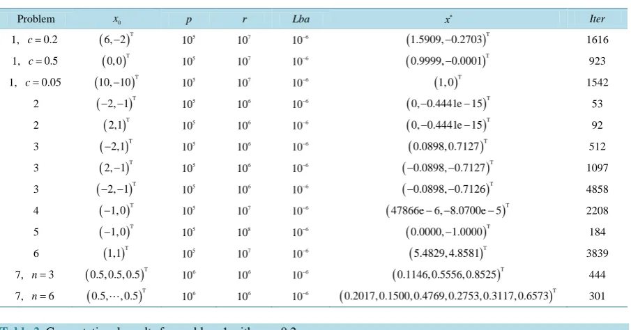
x until the algorithm terminates. The numerical results ofthe proposed algorithm are summarized in Table 1 for the above 7 problems.
Additionally, the proposed algorithm is compared with the algorithm presented in [11]. A series of minimizers obtained by the above two algorithms are recorded in Tables 2-14 for all testing problems.
Some symbols used in the following tables are given firstly.
0
x : The initial point which satisfies x0∈ Ω.
x∗: An approximate global minimizer obtained by the proposed algorithm.
Iter : The total number of function evaluations of f x
( )
and FFp( )
x until the algorithm terminates.The initial value of A is taken as 1 for all problems.
k: The iteration number in finding the k th local minimizer of the objective function;
k
x∗: The k th local minimizer;
k
f∗: The function value of xk
∗
[image:7.595.87.540.350.587.2]FABO : The algorithm proposed in this paper;
Table 1. Numerical results of all testing problems.
Problem x0 p r Lba x
∗
Iter
1, c=0.2 (6, 2− )T 5
10 7
10 6
10− (1.5909, 0.2703− )T 1616
1, c=0.5 ( )0, 0T 5
10 7
10 6
10− (0.9999, 0.0001− )T 923
1, c=0.05 (10, 10− )T 5
10 7
10 6
10− ( )1, 0T 1542
2 (− −2, 1)T 5
10 6
10 6
10− (0, 0.4441e 15− − )T 53
2 ( )2,1T 5
10 6
10 6
10− (0, 0.4441e 15− − )T 92
3 (−2,1)T 5
10 6
10 6
10− (0.0898, 0.7127)T 512
3 (2, 1− )T 5
10 6
10 6
10− (−0.0898, 0.7127− )T 1097
3 (− −2, 1)T 5
10 6
10 6
10− (−0.0898, 0.7126− )T 4858
4 (−1, 0)T 5
10 7
10 6
10− (47866e 6, 8.0700e 5− − − )T 2208
5 (−1, 0)T 5
10 8
10 6
10− (0.0000, 1.0000− )T 184
6 ( )1,1T 5
10 7
10 6
10− (5.4829, 4.8581)T 3839
7, n=3 (0.5, 0.5, 0.5)T 6
10 6
10 6
10− (0.1146, 0.5556, 0.8525)T 444
7, n=6 (0.5,, 0.5)T 6
10 6
10 6
10− (0.2017, 0.1500, 0.4769, 0.2753, 0.3117, 0.6573)T 301
Table 2. Computational results for problem 1 with c= 0.2.
FABO FABZ
k xk
∗
k
f∗ xk
∗
k
f∗
1 (5.7221, 1.8806− )T 2.5070 (5.7221, 1.8806− )T 2.5070
2 (3.7387, 1.2649− )T 0.6165 (4.7387, 1.7417− )T 1.6212
3 (0.5704, 0.0680− )T 0.1933 (4.7096, 1.3985− )T 1.3566
4 (1.5909, 0.2703− )T 5.6599e−009 (3.7387, 1.2649− )T 0.61647
5 (2.7380, 0.78836− )T 0.088673
Table 3. Computational results for problem 1 with c=0.5.
FABO FABZ
k xk
∗
k
f∗ xk
∗
k
f∗
1 (0.0420, 0.0948− )T 0.5175 (0.042023, 0.094772− )T 0.51745
2 (0.9999, 0.0000− )T 1.4998e−032 (0.99991, 1.2524e 4− − )T 2.2389e−7
3 (1.0000, 2.2205e 14− − )T 0
Table 4. Computational results for problem 1 with c=0.05.
FABO FABZ
k xk
∗
k
f∗ xk
∗
k
f∗
1 (8.7299, 3.2965− )T 9.0733 (8.7299, 3.2965− )T 9.0733
2 (7.7280, 2.8347− )T 6.5031 (7.7280, 2.8347− )T 6.5031
3 (4.7129, 1.4891− )T 1.5351 (6.7248, 2.3724− )T 4.3943
4 (1.8513, 0.4021− )T 8.4724e−010 (5.7198, 1.9162− )T 2.7434
5 (4.7129, 1.4891− )T 1.5351
6 (3.7305, 1.2306− )T 0.61844
7 (2.7300, 0.79341− )T 0.10216
8 (1.8513, 0.40209− )T 0
Table 5. Computational results for problem 2 with initial point
(
− −2, 1)
T.FABO FABZ
k xk
∗
k
f∗ xk
∗
k
f∗
1 (−1.7475, 0.8737− )T 0.2986 (−1.7476, 0.87378− )T 0.29864
2 (0, 0.4441e 15− − )T 1.9722e−031 ( )0, 0T 0
Table 6. Computational results for problem 2 with initial point
( )
2,1 . TFABO FABZ
k xk
∗
k
f∗ xk
∗
k
f∗
1 (1.7475, 0.8737)T 0.2986 (1.7476, 0.87378)T 0.29864
2 (0, 0.4441e 15− − )T 1.9722e−031 ( )0, 0T 0
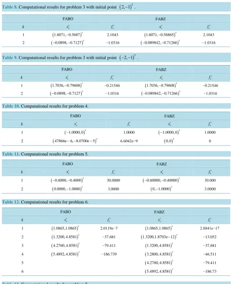
Table 7. Computational results for problem 3 with initial point
(
−2,1)
T.FABO FABZ
k xk
∗
k
f∗ xk
∗
k
f∗
1 (−1.6071, 0.5687)T 2.1043 (−1.6071, 0.56865)T 2.1043
2 (0.0898, 0.7127)T −1.0316 (0.089842, 0.71266)T −1.0316
FABZ : The algorithm proposed in reference [11].
Table 8. Computational results for problem 3 with initial point
(
2, 1−)
T.FABO FABZ
k xk
∗
k
f∗ xk
∗
k
f∗
1 (1.6071, 0.5687− )T 2.1043 (1.6071, 0.56865− )T 2.1043
2 (−0.0898, 0.7127− )T −1.0316 (−0.089842, 0.71266− )T −1.0316
Table 9. Computational results for problem 3 with initial point
(
− −2, 1)
T.FABO FABZ
k xk
∗
k
f∗ xk
∗
k
f∗
1 (1.7036, 0.79608− )T −0.21546 (1.7036, 0.79608− )T −0.21546
2 (−0.0898, 0.7127− )T −1.0316 (−0.089842, 0.71266− )T −1.0316
Table 10. Computational results for problem 4.
FABO FABZ
k xk
∗
k
f∗ xk
∗
k
f∗
1 (−1.0000, 0)T 1.0000 (−1.0000, 0)T 1.0000
2 (47866e 6, 8.0700e 5− − − )T 6.6042e−9 ( )0, 0T 0
Table 11. Computational results for problem 5.
FABO FABZ
k xk
∗
k
f∗ xk
∗
k
f∗
1 (−0.6000, 0.4000− )T 30.0000 (−0.60000, 0.40000− )T 30.000
2 (0.0000, 1.0000− )T 3.0000 (0, 1.0000− )T 3.0000
Table 12. Computational results for problem 6.
FABO FABZ
k xk
∗
k
f∗ xk
∗
k
f∗
1 (1.0865,1.0865)T 2.0119e−7 (1.0865,1.0865)T 2.8841e−17
2 (1.3200, 4.8581)T −37.681 (1.3200,1.8703e 12− )T −13.052
3 (4.2760, 4.8581)T −79.411 (1.3200, 4.8581)T −37.681
4 (5.4892, 4.8581)T −186.739 (3.2800, 4.8581)T −46.511
5 (4.2760, 4.8581)T −79.411
6 (5.4892, 4.8581)T −186.73
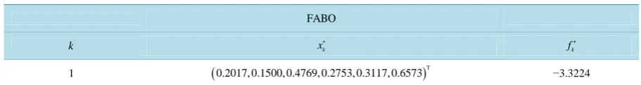
Table 13. Computational results for problem 7. FABO
k xk
∗
k
f∗
1 (0.3687, 0.1176, 0.2676)T −1.0008
Table 14. Computational results for problem 7 with n=6. FABO
k xk
∗
k
f∗
1 (0.2017, 0.1500, 0.4769, 0.2753, 0.3117, 0.6573)T −3.3224
also the lower computation cost will be; meanwhile, if the function value of the current local minimizer is closed to that of the global minimizer, then the sufficiently small Lba is necessary, while a relatively large initial value of A will cause increasing of number of iterations. Therefore, the initial value of A and Lba are needed to be selected accurately. The selection of Lba ensure the accuracy of the global minimizer, so that the sufficiently small Lba and appropriate small initial A should be selected or ρ contained in the algorithm is taken as small as possible.
5. Concluding Remarks
The filled function method is a kind of efficient approaches for the global optimization. The existing filled func- tions have some drawbacks, for example, some are non-differentiable functions, some contain more than one adjust parameter and some contain ill-condition terms and so on. These drawbacks may result in failure or diff- iculty of the algorithm in searching global optimal solution. In order to overcome these shortcomings, a new filled function with only one parameter is proposed in this paper. Although the proposed filled function is non- differentiable at some points, it can be approximated uniformly by a continuous differentiable function. The inherent shortcomings of the approximate function can be eliminated by simple treatment. The effectiveness of the new filled function method is demonstrated by numerical experiments on some testing optimization pro- blems.
Acknowledgements
This work was supported by the National Nature Science Foundation of China (No. 11161001, No. 61203372, No. 61402350, No. 61375121), The Research Foundation of Jinling Institute of Technology (No. jit-b-201314 and No. jit-n-201309) and Ningxia Foundation for key disciplines of Computational Mathematics.
References
[1] Ge, R.P. (1990) A Filled Function Method for Finding a Global Minimizer of a Function of Several Variables. Mathe-matical Programming, 46, 191-204. http://dx.doi.org/10.1007/BF01585737
[2] Ge, R.P. (1987) The Theory of Filled Function Method for Finding Global Minimizers of Nonlinearly Constrained Minimization Problems. Journal of Computational Mathematics, 5, 1-9.
[3] Wang, X.L. and Zhou, G.B. (2006) A New Filled Function for Unconstrained Global Optimization. Applied Mathe-matics and Computation, 174, 419-429. http://dx.doi.org/10.1016/j.amc.2005.05.009
[4] Wang, Y.-J. and Zhang, J.-S. (2008) A New Constructing Auxiliary Function Method for Global Optimization.
Mathematical Computer Modeling, 47, 1396-1410. http://dx.doi.org/10.1016/j.mcm.2007.08.007
[5] Liu, X. and Xu, W. (2004) A New Filled Function Applied to Global Optimization. Computer and Operation Research,
31, 61-80. http://dx.doi.org/10.1016/S0305-0548(02)00154-5
[6] Liu, X. (2004) The Barrier Attribute of Filled Functions. Applied Mathematics and Computation, 149, 641-649.
http://dx.doi.org/10.1016/S0096-3003(03)00168-1
[7] Dixon, L.C.W., Gomulka, J. and Herson, S.E. (1976) Reflections on Global Optimization Problem, Optimization in Action. Academic Press, New York, 398-435.
[8] Liang, Y.M., Zhang, L.S., Li, M.M. and Han, B.S. (2007) A Filled Function Method for Global Optimization. Journal
of Computational and Applied Mathematics, 205, 16-31. http://dx.doi.org/10.1016/j.cam.2006.04.038
[9] Ling, A.-F., Xu, C.-X. and Xua, F.-M. (2008) A Discrete Filled Function Algorithm for Approximate Global Solutions
of Max-Cut Problems. Journal of Computational and Applied Mathematics, 220, 643-660.
http://dx.doi.org/10.1016/j.cam.2007.09.012
Prob-lems. Journal of Optimization Theory and Applications, 119, 459-484.
http://dx.doi.org/10.1023/B:JOTA.0000006685.60019.3e
[11] Zhang, L.-S., Ng, C.-K., Li, D. and Tian, W.-W. (2004) A New Filled Function Method for Global Optimization.