Mathematical Model of a Photovoltaic Grid Connected Two Area Power System

(1)

Mathematical Model of a Photovoltaic Grid Connected Two-Area Power

System

Samar Emara

1

_{, Abdulla Ismail}

2

_{, Ali Sayyad}

3

1_{Graduate Student, Department of Electrical Engineering and Computing Sciences, RIT, Dubai, UAE} 2_{Professor, Department of Electrical Engineering and Computing Sciences, RIT, Dubai, UAE}

3_{Lecturer, Department of Electrical Engineering and Computing Sciences, RIT, Dubai, UAE}

***Abstract

-In this paper, a mathematical model of a PV grid connected two-area power system with 45% penetration level is presented. The models of the thermal power system and the PV system are explained as well as the connection between both systems. In addition, the system frequency errors, due to various cases of load changes in this PV connected power grid are studied using MATLAB/Simulink simulation.

Key Words: power, photovoltaic, PV, renewable, mathematical, model, Simulink, MATLAB.

1.INTRODUCTION

As the contribution of renewable energy is becoming an essential part of the power generation, it is of critical importance to study the effects of this increased penetration of the renewable energy sources on the power system and the potential problems associated with it. The load frequency control (LFC) is one of the main points to be considered in the study of this interconnected system. [1] In order to be able to design controllers for this interconnected system, a reliable mathematical model should be established for both the thermal power system and the PV system and their interconnection.

Section 2 of this paper presents the model of a two-area power system connected to PV system. The detailed explanation relative to the mathematical model of the PV system along with its corresponding calculations are explained in section 3. In section 4, by combining the two systems studied in sections 2 and 3, the overall PV grid connected two- area power system has been constructed and the effect of PV penetration on the frequency behavior of the power system. Moreover, the frequency response due to various load changes are also presented through this section.

2.MODELING THERMAL POWER SYSTEMS

A typical thermal power plant consists of a governor to monitor and measure the system speed changes and to control the valve, a turbine which transforms the input energy (in this case coming from the steam) into mechanical energy that is the input to the generator, which transforms this mechanical energy into electrical energy. The reheater

makes the system more efficient as it reheats the steam to keep the same high temperature of the steam that enters the governor. [2]

In this section the specific mathematical model of each area has been presented along with the response of each area in this system without controllers. The integral controller is required in both areas, since, in general, one of the criteria to be met for the system frequency in a thermal power system, is a zero steady state error (△f=0 change of frequency=0; i.e. frequency remains constant at 50Hz). Note that as the integral controller adds one state variable to the model of the system, it has been included to the models that will follow.

2.1Mathematical Model of Area 1

[image:1.595.305.572.475.609.2]

The state model of the first area in the given thermal power system containing integral controller is presented here. Table 1 shows the parameters that were used in this modeling. Moreover, the block diagram corresponding to this model is presented in Figure 1.

Table -1:Parameters of the thermal power system

Parameter Definition Value

Governor time constant 0.08

Droop 2.4

Turbine time constant 0.3

Reheater time constant 10

Reheater gain 0.5

Generator time constant 20

Gain constant 120

The change in the power of the load △Pload is acting as the

disturbance input to this area. Using x1 to x5 as the state variables of the system, the following state equations (Equations 1-5) represent area 1. Clearly the additional state variable is due to presence of the integral controller. The purpose of adding this integral controller is due to its positive impact on the system frequency response improvement which will be observed when it comes to the discussions of the system respond. A value of integral controller gain Ki=0.6

(2)

Accordingly, the state model of the thermal power system with an integral controller becomes the following (Equations 6 and 7).

2.2 Mathematical Model of Area 2

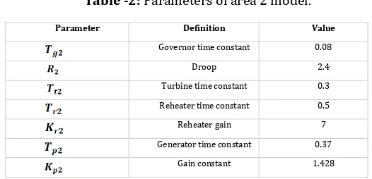
Table -2: Parameters of area 2 model.

Parameter Definition Value

Governor time constant 0.08

Droop 2.4

Turbine time constant 0.3

Reheater time constant 0.5

Reheater gain 7

Generator time constant 0.37

Gain constant 1.428

Table 2 shows the parameters corresponding to the state model of area 2 and Figure 2 shows the block diagram of this area. The state space equations of this power system have been calculated as follows (Equations 8-12). This model includes the integral controller in order to eliminate the

steady state error.

(1)

[image:2.595.34.582.49.214.2]

(2)

Fig -1: Block diagram of area 1.

(3)

(4)

(5)

(6)

(7)

Fig -2: Block diagram of area 2 in the thermal power system.

(8) (9)

[image:2.595.304.567.259.386.2] [image:2.595.35.566.461.756.2]

(3)

In matrix form, we have

3.PV SYSTEM MODEL

In order to connect a PV array to a thermal power system, having the knowledge and applying the rules of power electronics would be of importance. [3 & 4] After obtaining the power output from the PV array, the first stage of this connection with the thermal power system is to use the boost converter. It increases the voltage to a suitable level, so that this voltage can be used as an input for the second stage of diagram which is the inverter. The inverter produces an AC current in order to be compatible with the AC nature of the power input applied to the grid and to be synchronized with its voltage and current. [3] The input to the PV system connected to the grid is the output of the PV array which is a DC current.

The system in this work consists of 150 30kW connected arrays with a constant voltage source of 6kV at the PV array side. [5] The PV is at a low voltage and low power side, usually in inverter-based PV systems connected to grids, with the power in order of 1kW to a few MW. [6]

The maximum power point (MPP) is the point at which the maximum output power is obtained. It occurs only at a certain voltage value. [7] The MPP of this connection of solar arrays is at which gives an MPP of 4.5MW. This is suitable for the current application because the maximum load of the thermal power system is 10MVA.

The output of the solar cell/array is always DC. If this output is measured for a long period of time (i.e. hours) is nonlinear. However, when it’s measured in terms of seconds (which is the period required to be considered for designing controllers to the system) will be resulted to a constant DC – shape voltage. In fact, even when a change occurs on the voltage, over a long period of time due to a change of temperature or solar irradiance, it varies from a certain DC

value to another DC value (different amplitude but it remains a constant DC).

Moreover, because the PV array acts as a simple PN junction diode and the output is a DC current, [8 & 9] the ideal PV array circuit has no order; i.e. does not add state variables to the system model. That is why the output from that solar array is taken directly into the PV system, as it will not affect the calculations of the state model.

[image:3.595.31.294.102.347.2]

Before going into the details of each block, all the parameters that will be used in the PV systems are summarized in Table 3. Figure 3 shows the process in the photovoltaic system designed for the grid studied in this paper.

Table -3: Symbols used in the PV system model.

Symbol Definition

Output voltage from the PV array (V)

Voltage after the DC-DC boost converter (compatible with grid voltage) (V)

The gain between the DC voltage and the AC voltage in the system

Boost converter gain

Output current from the PV array (amp)

Current after the DC-DC boost converter in the PV system (amp)

The inverted current in the PV system (amp)

Instantaneous power of the PV system (W)

Average power of the PV system (W)

Phase grid voltage (V)

System frequency (rad/s)

Fig. -3: General block diagram of the connection between the PV array and the grid.

Considering Figure 3, is shows that the first stage in the connection between a PV system and power system is the DC-DC boost converter is used in order to connect PV system to the grid. In the ideal case, this converter is just a gain. To obtain this gain, it is important to know the total gain required between the DC voltage and the amplitude of the final AC voltage (m) as shown in Equation 15.

(11)

(12)

(13)

(14)

[image:3.595.302.577.275.618.2]

(4)

The value of is ideally less than 0.866, and it has been chosen in this model to be 0.7. The PV system operates at a

constant DC voltage , while the output current

and power of the PV arrays change according to the irradiance of the sun and the temperature. [5] Since this DC value is constant, by choosing for this specific system, the amplitude of the AC voltage will also remain constant, leaving the AC current and power to vary along with the changes.

This can now be used in the calculations to find the value of the voltage required after the boost converter as shown in Equation 16. The photovoltaic system is applied at the low voltage side of the grid and the RMS value of the grid line voltage of the conventional system that is considered here is 11kV. This means that the grid phase voltage is kV. This is the value that will be used since in this photovoltaic system only one phase (phase A) is considered. There are two other phases (B and C) providing the system with the same power but with a certain phase shift.

Accordingly, the boost converter gain can be calculated as

Since , therefore, assuming an ideal DC-DC

boost converter (with the switching frequency much higher than the system dynamics), the gain for the boost converter is representing the first transfer function (Equation 18):

The next stage is the DC-AC inverter which converts this DC current to an AC current that will be suitable for the connection with the conventional AC based power system. The transfer function can be obtained by dividing the Laplace transform of each term.

The AC current ( is simply given by the form , and this has a Laplace transform of ,

where . Similarly,

(the current after the boost converter) is a DC value so it has the Laplace transform of . Therefore, the transfer function of the second block (current inverter) is Equation 19:

Figure 4 shows the inverted current resulting from the current inversion stage in the model presented. Two periods in the graph are between 45ms and 5ms which is 40ms. Therefore, the frequency of the current is 2/40ms=50Hz, which is the system’s frequency as expected.

Fig. -4: Current Inversion from DC (after boost converter) to AC with 50Hz (system frequency).

The third stage is to convert this current to instantaneous power to match the output of the thermal power system. Thus, the input from the PV system to the grid should also be in terms of power. The transfer function of this block can be obtained similar to the method of obtaining . First, the instantaneous power p(t) is given by Equation 20.

The gain is an impedance which is is purely resistive. Taking the Laplace transform of Equation 20 gives Equation 21.

where is the same expression obtained previously. Therefore, the transfer function for the conversion from AC current to instantaneous power is Equation 22:

The instantaneous power has double the frequency of the inverted current because the equation of instantaneous power is given by the multiplication of two cosine waves (the current and the voltage) each of which has a frequency of 50Hz, and by the trigonometric identities, this produces a cosine wave of double the frequency. Thus, a frequency of (16)

(17)

(18)

(19)

(20)

(21)

[image:4.595.310.558.172.337.2]

(5)

[image:5.595.35.285.165.357.2]

100Hz can be seen on the graph shown in Figure 5 for the instantaneous power. One period occurs between 2.6ms and 12.6ms, i.e 10ms giving a frequency of 1/10ms=100Hz. The voltage and the current are in phase, therefore there is no reactive power going from the PV array to the grid. [3]

Fig. -5: Instantaneous power from the photovoltaic system (100 Hz).

Since the load in photovoltaic systems is purely resistive, the instantaneous power graph is expected to be completely offset in the positive y-axis (above the x-axis) which is the case in Figure 5. This explains why the instantaneous power has double the amplitude (9MW instead of 4.5MW), because

the real negative peak of the original sine wave is at -4.5MW, but with the offset that occurred, the negative

amplitude shifted to the positive side making the -4.5 start from 0 and the 4.5 peak to shift to 9MW.

However, the required output power of the PV system that will be a second input to the thermal power system is the average power not the instantaneous power in order to make them compatible with each other. [10] Thus, the last stage here is to convert the instantaneous power to average power. The equation for the average power in the time domain is Equation 23:

which is expected since the load is purely resistive, and the average power would be a constant. The Laplace transform of the average power is

[image:5.595.314.558.405.590.2]

To obtain the transfer function of the conversion from instantaneous power to average power after simplification (Equation 25), we have

[image:5.595.37.569.575.794.2]

Figure 6 shows the final output of the PV system which is the MPP average power (4.5 MW) as expected because this is half of the amplitude of the offset instantaneous power graph. If the power was not purely resistive, then the real power will be less than 4.5MW because part of the graph of the instantaneous power will be below the x axis depicting reactive power. Connecting all the above blocks together leads to the full PV system which is shown in Figure 7.

Fig. -6: Average power output of the PV (second input to thermal power system).

(24)

(25)

(23)

(6)

In order to obtain the state model of this PV system, the controllable canonical form method is chosen and applied as follow. Starting with the DC-AC inverter block, the controllable canonical form is obtained from the following state equations (Equations 26-28). in the following equations represent the input to each sub-system.

Giving the following state model (Equations 29 and 30)

[image:6.595.309.566.87.282.2] [image:6.595.312.555.347.490.2]

Realizing this state model into a block diagram is shown in Figure 8.

Fig -8: DC-AC inverter block to obtain controllable canonical form.

As to , the same steps are applied to obtain the state Equations (Equations 31-35)

Leading to the state model (Equations 36 and 37), and Figure 9 shows the detailed blocks in the canonical form for .

Fig. -9: Instantaneous power blocks to obtain controllable canonical form.

Similarly, is also dealt with in the same manner with state Equations (38-40)

[image:6.595.22.272.366.452.2]

In matrix form, we have

[image:6.595.317.560.525.631.2]

Figure 10 shows the detailed blocks in canonical form.

Fig. -10: Average power block to obtain controllable canonical form.

Combining all of these state models for the sub-blocks into one state model gives the following state matrix (matrix 43). As to , since it is only a constant connected to the input, it is accounted for in the B matrix (matrix 44). C and D matrices are shown in matrices 45 and 46.

(27)

(28)

(29)

(30)

(31)

(32)

(33) (34)

(35)

(36)

(37)

(38)

(39)

(40)

(41)

(7)

C=

D=

Notice that these sub-blocks are interconnected, therefore, these extra connections need to be accounted for. To get these values of the interconnection, some state equations needed to be modified. The modified state Equations 47 and 48 demonstrate how these values were obtained. The term here in the full state matrix represents the input of the photovoltaic system rather than the input of each sub-block separately.

Simplifying Equation 47 gives:

In addition, to get the D matrix, the following calculation has been done by tracking how the output is directly related to the input. It can also be obtained directly from the final equation.

An additional model that was also useful in some calculations is the full transfer function of the PV system

shown in Equation 51, where ; i.e. the output

of the PV array which is the input to the PV system.

4.PV GRID CONNECTED TWO-AREA POWER SYSTEM

This section presents the connection of both the photovoltaic system and the single-area thermal power system that were previously explained.

Note that during all of the mathematical calculations, “per unit (p.u)” is used for the element of power, which is why the power in Figure 7 is given in p.u. MVA. This is due to the fact that the values in the power system given by the transfer functions will result in a value of power in p.u. automatically. Therefore, in order to make the units compatible with each other before connecting both systems, the output power of the photovoltaic system also needs to be converted to per unit. Per unit system is a way of calculation so that all the values obtained from a certain system can be expressed as a ratio of one common value (which is the base value). [11]

The base value is the reference with which all other values in the system are compared. The base value of this thermal power system is 10MVA which is the rating of the generator. [11] Thus, compared with that scale, a change in load of 1p.u. is equivalent to a change of 10MW and a change of 0.5p.u. is equivalent to a change of 5MW (50% change in load).

The base load of the power system is considered 10MVA in terms of apparent power, however, since the load is purely resistive, it means that all the apparent power is real power, and there is no reactive power. That is why it can be considered that the base value is 10MW. The average output power of the PV system is also compared to this base value of 10MW. For example, an average output power of 4.5MW

in the PV system is equivalent to and this

is the value at MPP. in the design of the PV system is modified according to this calculation to obtain the final output of the PV system ( ), which by its turn becomes the second input to the thermal power system, besides the first input which is the change in the power of the load

The penetration level of PV in the conventional thermal power system also needs to be determined before the connection. PV penetration is defined as the rated PV capacity as a ratio to the total capacity of the grid. [5] The photovoltaic capacity is 4.5MVA=4.5MW (0.45 p.u.) and the total capacity of the system grid is 10MVA (1 p.u.). Therefore, there is a 45% PV penetration level in the system under study.

According to these calculations and the previously explained models of the PV system and the two-area thermal power system, the connection is now possible.

(43)

(44)

(45) (46)

(47)

(48)

(49)

(50)

(8)

Area 1 and area 2 are connected first then connected to the PV system. For the connection of these areas together, there are 5 state variables from the first area and 5 state variables from the second. However, the interconnection adds one more state variable because of the tie-line power change giving a total of 11.

As to the full model of the two-area system in terms of thermal power system, combining Equations 1-5 and 8-12 along with the following modifications (demonstrated in Equations 52-56) give the state model accounting for the interconnected parts between both areas. The state model of the two-area system connected to PV is shown in matrices 57-60.

The system state matrix (A)=

After the connection of this two-area model with the PV system, each area has two inputs; the input of change of load power and another input from the PV system connected to the grid. Therefore, for this interconnected system, it has four

inputs ( , , & ) and two outputs

which are the change in frequency of area 1 ( ) represented by the 1st_{state variable and the change in}

frequency of area 2 ( ) represented by the 6th_state

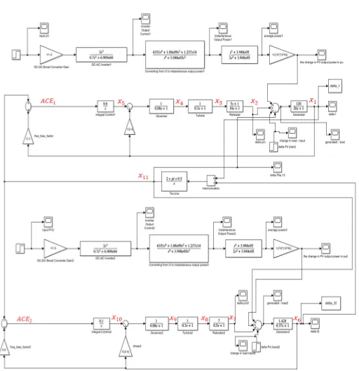
variable. Figure 11 shows both systems after being connected.

The controllability and observability of the system have also been checked. The rank of both the controllability matrix and the observability matrix is equal to 11 which is the same as the number of state variables, therefore, the two-area system is controllable and observable.

As to the stability of the two-area system, the eigenvalues are: -12.8774, -11.0897, -8.4731, -0.2412+ 5.7803i,

-0.2412-5.7803i, -0.2479+2.8600i, -0.2479 - 2.8600i, -2.5267, -0.2152+0.1814i, -0.215-0.1814i & -0.1439. All the poles

(eigenvalues) are negative, therefore, the system is stable.

Figure 12 shows the response of the two-area system without any controller (without even the integral controller), Figure 13 and Figure 14 show the response of both outputs in this system with integral controller for various changes in load (reasonable change in load and an extreme change in load (50%)).

It is observed from Figure 12 that without using the integral controller the steady state error does not diminish, which is not desired in standard applications. When including the integral controller, the steady state error requirement is met. Additional controllers need to be designed for the system to meet the other standard specifications of the settling time and the undershoot in power systems.

Fig -12: Response of the two-area system without any controller due to 50% increase in load. (52)

(53)

(54) (55) (56)

(57)

(58)

(59)

(9)

[image:9.595.46.558.99.628.2]

Fig -11: Block Diagram of the two-area system connected with the PV system.

(10)

[image:10.595.36.304.56.299.2]

system with integral controller) for 50% increase in load.

Fig -14: Change of frequency of both areas (for the system with integral controller) for reasonable load.

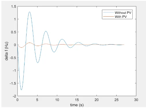
One of the objectives in this paper is also to determine the effect of the connection of a photovoltaic system to a thermal power system on the frequency of the system. This would be helpful in designing a controller that takes this effect into consideration. Figure 15 shows the response of the system before and after connecting it to a PV system with a 100% change in load, and Figure 16 for less than 50% load change. Both figures (15 and 16) show the response of area 1 in the two-area system. Table 4 also summarizes the responses to notice the effect of PV penetration on the system frequency. It can be clearly noticed that the effect of connecting PV to the system is in fact positive, because it helps the power system to match the load demand. Other research has also shown that the more the penetration of the photovoltaic array output in the conventional power grid, the less the

[image:10.595.312.562.181.364.2]

deviation of the frequency output [12 & 13]. In [8], it is demonstrated that since PV only provides real power, then any shading will only affect the frequency negatively at the transmission level, not at the utility grid side. Therefore, the effect of PV connection to the grid has a positive effect on the frequency.

Fig. -15: Comparison between responses of the system connected and unconnected to the PV system (100% load

increase).

Fig. -16: Response of the system with and without PV (for a reasonable change in load).

Table -4: Comparison for the responses of the thermal power system with and without the connection to PV.

Without PV (100%

load)

With PV (100%

load)

Without PV

(20% load) (20% load) With PV

Settling Time (s) 19.7165 19.7165 19.7165 19.7165

Undershoot (Hz) -3.679 -2.0239 -0.11039 -1.7663

SSE (Hz) 0 0 0 0

[image:10.595.308.561.425.613.2]

(11)

This positive effect on the undershoot could be explained as follows. The mechanical power generated from the thermal system equals the power of the load added to the power loss but subtracted from the power of the photovoltaic system as in Equation 61. [6]

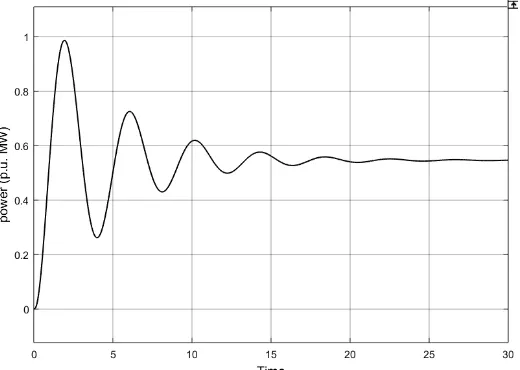
[image:11.595.31.291.426.611.2]

Thus, the PV system reduces the pressure on the thermal power system. This is because, in the graph (without PV) in Figure 15, had to provide the system with the full power demand (1p.u.) which is why it settles down at this value. However, after the connection with PV (non-dispatchable generator), (dispatchable generator, i.e. the one in the thermal power system) is now providing only the remaining part of what the PV could not provide, keeping the power flow unchanged. [12] Therefore, it settles at a value less than 1p.u. as shown in Figure 17, i.e., the load is now distributed between the PV system and the thermal power system. is a DC value as explained earlier and does not contribute to more oscillations nor takes time to reach the steady state. Since thismakes provide for less load, it has a smaller undershoot. These factors affect the output ( ) positively by reducing the undershoot of the system, but not affecting the settling time neither positively nor negatively.

Fig. -17: The mechanical power settling at a value less than that of the load change due to the penetration of PV. Another observation from the effect of the connection of PV to the system is that there is no difference in the settling time with the changes in load in the PV-connected thermal power system. The undershoot is the parameter that is improved. Thus, the PV system has no effect on the settling time of the deviation of frequency, but just on the undershoot of the system.

Regarding the control of this PV grid connected two-area power system, it is to be noted that the source in the PV arrays (which is the sun) cannot be controlled unlike the

thermal power systems where the amount of steam can be controlled based on the demand. [14] However, control can be done in the photovoltaic system connection to the grid in the DC-AC inverters. [7] It increases the efficiency of the system and ensures the operation at MPP. The Maximum Power Point Tracker (MPPT) is the controller that tracks the maximum power point and ensures that the system operates at this point most of the time. [9]

Another control possibility in the PV system is the following case. When the input to the grid due to PV is more than the load demand at a certain point, power is inverted and is injected back to the AC side. It can also be stored in a battery if the system is connected to one. [4] The photovoltaic system can be controlled if there is a battery connected to it to improve the frequency control of the system. [15] However, controllers can be easily applied to the thermal power system in this interconnected system rather than to the PV in order to do the Load Frequency Control (LFC).

5.CONCLUSION

This paper presented a model of a PV system connected to a two-area thermal power plant with penetration level of 45%. The mathematical details of the full model have been explained. The effect of this connection on the power system turned out to be positive on the undershoot and had no effect on the settling time. This was proved by simulation results. The response of the full system was shown for various loads. Only an integral controller has been incorporated into the model of the system to ensure a steady state error of zero. In power systems, there are usually strict requirements for the undershoot and settling time, which would require the design of additional advanced controllers.

ACKNOWLEDGEMENT

The authors wish to thank RIT Dubai for the support.

REFERENCES

[1] A. Ikhe, A. Kulkarni, D. Veeresh, “Load frequency control

using fuzzy logic controller of two-area thermal-thermal power plant,” International Journal of Emerging Technology and Advanced Engineering, ISSN 2250-2459, vol. 2, issue 10, October 2012.

[2] A. Monti and F. Ponci, “Electric power systems”,

Intelligent Monitoring, Control, and Security of Critical Infrastructure Systems Springer, 2015. DOI 10.1007/978-3-662-44160-2_2)

[3] M. Alam and F. Khan, “Transfer function mapping for a

grid connected PV system using reverse synthesis technique,” in 14th Workshop on Control and Modeling for Power Electronics (COMPEL)-IEEE, 2013.

[4] X. Liu, P. Wang, P. Loh, “A hybrid AC-DC microgrid and

its coordination control,” IEEE Transactions on Smart Grid, vol. 2, no. 2, June 2011.

[5] S. Pourmousavi, A. Cifala, and M. Nehrir, “Impact of high

(12)

Symposium (NAPS)-IEEE, September 2012. DOI 10.1109/NAPS.2012.6336320

[6] H. Bevrani, A. Ghosh, G. Ledwich, “Renewable energy

sources and frequency regulation: survey and new perspectives,” IET Renewable Power Generation, vol. 4, issue 5, pp. 438–457, February 2010. DOI: 10.1049/iet-rpg.2009.0049

[7] N. Cao, Y. Cao, J. Liu, “Modeling and analysis of grid

connected inverter for PV generation,” in proceedings of the 2nd International Conference on Computer Science and Electronics Engineering (ICCSEE), Paris, 2013.

[8] Z. Kamaruzzaman, A. Mohamed, H. Shareef, “Effect of

grid-connected photovoltaic systems on static and dynamic voltage stability with analysis techniques – a review,” in Przeglad Elektrotechniczny, June 2015.

[9] S. Yang, “Solar energy control system design,” Master of

Science thesis, KTH Information and Communication Technology, Stockholm, Sweden, 2013.

[10] K. Arulkumar, K. Palanisamy & D.Vijayakumar, “Recent

Advances and Control Techniques in Grid Connected Pv System – A Review”, International Journal of Renewable Energy Research, Vol.6, No.3, 2016.

[11] “The utility edge,” Power System Engineering Inc., USA,

2015.

[12] Y. Liu, L. Zhu, L. Zhan, J. Gracia, T. King, Y. Liu, “Active

power control of solar PV generation for large interconnection frequency regulation and oscillation damping,” International Journal of Energy Research, vol. 40, pp. 353–361, June 2015. [online]. Available: Wiley Online Library (wileyonlinelibrary.com) DOI: 10.1002/er.3362

[13] A. Abdlrahem, G. Venayagamoorthy, K. Corzine,

“Frequency stability and control of a power system with large PV plants using PMU information,” in North American Power Symposium (NAPS) IEEE, September 2013.

[14] E.F. Camacho, M. Berenguel, F .R. Rubio, Advanced

Control of Solar Plants, London: Verlag London Springer, 1997.

[15] P. Tielens, D. Hertem, “Grid inertia and frequency

control in power systems with high penetration of renewables,” Semantic Scholar, 2012.

BIOGRAPHIES

Samar A. Emara Born in 1994.

Graduated with BSc in Electrical Engineering from the Petroleum Institute, Abu Dhabi in 2016. Currently doing MSc in Electrical Engineering (in control systems) at RIT Dubai.

Worked as a teaching assistant for the academic year (2016-2017) at RIT Dubai and is currently a full time Master

student. Samar is a student member of IEEE and has filed a patent of the project entitled (Design of Nanomagnetic Tagging and Monitoring System) in 2016.

Abdulla Ismail Professor of

Electrical Engineering. Emirati citizen, Born in Sharjah. BSc (‘80), MSc (’83), and PhD (’86) in Electrical Engineering from University of Arizona, USA. 1st Emirati to hold a PhD in Engineering. Has over 30 years of teaching and research experience at UAE University (ALAIN) and RIT Dubai.

Worked as Vice Dean of College of Engineering, Advisor to the Vice Chancellor at UAE University. Worked in Education and Technology management Dubai Silicon Oasis and Emirates Foundation. Teaching and research interests in Control and Power systems, intelligent systems, smart grids, renewable energy systems modeling and control.

Coauthored two books; desalination technology in the UAE and Contemporary Scientific Issues. Published over 90 referred technical papers in local and international journals and conferences. Won Emirates Energy Award (Education and Energy Management), 2015. Won several UAEU awards for University and Community service. Won the Fulbright scholarship, USA Government. A senior member of IEEE. A member of Dubai KHDA University Quality Assurance International Board, Chair of the Zayed Future Energy Prize (Global High Schools Committee), Chairman of AURAK Engineering Advisory Council.

Ali A. Sayyad PhD in Systems and Control Engineering, City, University of London, UK. Research interests include control system analysis and design including modelling and optimization techniques in both linear and nonlinear cases and Robust control applications

Holds more than Six years of experience in industrial field, working as an electrical and/or Control engineer. Since 2013, he has also been a member of STEM organization. Dr. Sayyad joined the Department of Electrical Engineering as an Electrical Lecturer, at Rochester Institute of Technology Dubai in September 2017.