R E S E A R C H
Open Access
Two spectral gradient projection methods for
constrained equations and their linear
convergence rate
Jing Liu
1?and Yongrui Duan
2*?*Correspondence: [email protected]
2School of Economics and
Management, Tongji University, Siping Street, Shanghai, 200092, P.R. China
?Equal contributors
Full list of author information is available at the end of the article
Abstract
Due to its simplicity and numerical efficiency for unconstrained optimization problems, the spectral gradient method has received more and more attention in recent years. In this paper, two spectral gradient projection methods for constrained equations are proposed, which are combinations of the well-known spectral gradient method and the hyperplane projection method. The new methods are not only derivative-free, but also completely matrix-free, and consequently they can be applied to solve large-scale constrained equations. Under the condition that the underlying mapping of the constrained equations is Lipschitz continuous or strongly monotone, we establish the global convergence of the new methods. Compared with the existing gradient methods for solving such problems, the new methods possess a linear convergence rate under some error bound conditions. Furthermore, a relax factor
γ
is attached in the update step to accelerate convergence. Preliminary numerical results show that they are efficient and promising in practice.Keywords: constrained equations; spectral gradient method; projection method; global convergence
1 Introduction
In this paper, we consider the problems of finding a solution of the following constrained equations, denoted byCES(F,C),
Fx∗= subject to x∗∈C, ()
whereF:C→Rnis a given continuous nonlinear mapping andCis a nonempty closed convex set ofRn. Obviously, whenC=Rn, () reduces to the nonlinear equations, which is
intensively studied by many scholars. The constrained system of equations () appears in wide variety of problems in applied mathematics, and some important problems, such as economic equilibrium problems [], power flow equations [], and chemical equilibrium systems [], can be reformulated as a problem of the kind ().
Among various numerical methods for solvingCES(F,C) [–], the gradient projection methods (GPMs) are the most efficient, especially when the projection onto the feasible setCis easy to implement. For example, whenCis the nonnegative orthant, or a box, or a ball, GPMs require the lowest computational cost. In addition, the GPMs are also
the simplest, because they do not need to store any matrix during the iteration process. Therefore, they are completely matrix-free, and consequently, they can be applied to solve large-scaleCES(F,C).
It is well known that the spectral gradient method [, ] and the conjugate gradient method [] are two efficient methods for solving large-scale unconstrained optimiza-tion problems due to their simplicity and low storage. Recently, combined with the pro-jection technique, they are extended to solve constrained equationsCES(F,C) by some scholars [, ]. In [], Yuet al.proposed a spectral gradient projection method for solv-ing monotoneCES(F,C), which can be applied to nonsmooth constrained equation, and works quite well even for large-scaleCES(F,C). Quite recently, Liuet al.[] developed two unified frameworks of some sufficient descent conjugate gradient projection methods for solving monotoneCES(F,C), which are also applied to solve large-scale nonsmooth con-strained equations. However, the convergence rate issue of the methods in [, ] is not investigated. Therefore, whether they have a linear convergence rate is an open problem. Can we design a spectral/conjugate gradient projection method with a linear convergence rate forCES(F,C)? In this paper, we answer this question positively for spectral gradi-ent projection method. Note that, in [], Dai and Liao proved a nice conclusion for the spectral gradient method. In fact, they established theR-linear convergence of the spec-tral gradient method for strongly convex quadratics of any number of dimensions, and they also proved the locallyR-linear convergence for the general objective function. Ob-viously, the general minimization problem discussed in [] is equivalent to the system of nonlinear equations under some mild conditions. However, for the system of constrained nonlinear equations, we shall establish the locallyR-linear convergence of the spectral gra-dient method in this paper. Therefore, our result extends the conclusion in [] in some sense.
In fact, in this paper, motivated by the projection methods in [, ] and the spectral gradient method in [], we propose two spectral gradient projection methods for solv-ing nonsmooth constrained equations, which can be viewed as combinations of the well-known spectral gradient method and the famous hyperplane projection method, and they possess a linear convergence rate under some error bound conditions. The remainder of this paper is organized as follows. In the next section, we describe the new methods and present their global convergence analysis. The linear convergence rates of the new meth-ods are established in Section . Numerical results are reported in Section . Finally, some final remarks are included in Section .
2 Algorithm and convergence analysis
First, we denotex=√xxas the Euclidean-norm. LetC∗ denote the solution set of
CES(F,C). Throughout this paper, we assume that:
(A) The solution setC∗is nonempty. (A) The mappingF(·)is monotone onC,i.e.,
F(x) –F(y),x–y≥, for allx,y∈C.
(A) The mappingF(·)is Lipschitz continuous onC,i.e., there is a positive constantL such that
(A) The mappingF(·)is strongly monotone onC,i.e., there is a positive constantη
such that
F(x) –F(y),x–y≥ηx–y, for allx,y∈C. () Obviously, (A) implies (A), and from () and the Cauchy-Schwartz inequality, we have
F(x) –F(y)≥ηx–y, for allx,y∈C. ()
Then letPC(·) denote the projection mapping fromRnonto the convex setC,i.e.,
PC(x) =argmin
x–y|y∈C,
which has the following nonexpansive property:
PC(x) –PC(y)≤ x–y, ∀x,y∈Rn. ()
Now, we review the spectral gradient method for the unconstrained minimization prob-lem:
minf(x), x∈Rn, ()
wheref :Rn→Ris smooth and its gradient is available. The spectral gradient for solving () is an iterative method of the form
xk+=xk–αk∇f(xk),
whereαkis a step size defined by (see [])
αIk=s
k–yk–
yk–yk–
or αkII=s
k–sk–
sk–yk–
, ()
in whichsk–=xk–xk–,yk–=∇f(xk) –∇f(xk–). The step sizes () are called
Barzilai-Borwein (BB) step sizes, and the corresponding gradient methods are spectral gradient methods. The spectral gradient with step sizeαIIk has been extended to solve the con-strained equations () by Yuet al.[], however, as discussed in the Introduction, we do not know whether the method in [] possesses the linear convergence rate. In the follow-ing, we will extend the spectral gradient with step sizeαI
k andαIIk to solve constrained
equations () by some new type Armijo line searches, and we propose two spectral gra-dient projection methods, which are not only globally convergent, but also have a linear convergence rate.
The spectral gradient projection methods are stated as follows.
Algorithm .
Step . Set an arbitrary initial point x∈C, the parameters <ρ< , <σ <r< ,
<γ< , and <βmin<βmax. Set the initial step sizeβ= and setk:= .
Step . Computedkby
dk=
–F(xk), ifk= ,
–θkF(xk), ifk≥,
()
where
θk= sk–yk–
yk–yk–
, ()
which is similar toαIkdefined in (),yk–=F(xk) –F(xk–), butsk–is defined by
sk–=xk–xk–+ryk–,
which is different from the standard definition ofsk–. Stop ifdk= ; otherwise, go to
Step .
Step . Find the trial pointzk=xk+αkdk, whereαk=βkρmkwithmkbeing the smallest
nonnegative integermsuch that
–F(xk+αkdk),dk
≥σF(xk). ()
Step . Compute
xk+=PC
xk–γ ξkF(zk)
, ()
where
ξk=
F(zk),xk–zk
F(zk)
. ()
Choose an initial step sizeβk+such thatβk+∈[βmin,βmax]. Setk:=k+ and go to Step .
Algorithm .
Step . Set an arbitrary initial pointx∈C, computeL, the Lipschitz constant ofF(·),
choose the parameters <ρ< , <r< , <σ<r/(L+r), <γ < , and <β
min<βmax.
Set the initial step sizeβ= and setk:= .
Step . IfF(xk) = , then stop; otherwise, go to Step .
Step . Computedkby
dk=
–F(xk), ifk= ,
–ϑkF(xk), ifk≥,
where
ϑk= sk–sk–
sk–yk–
,
which is similar toαIIk defined in (),sk–=xk–xk–, butyk–is defined by
which is different from the standard definition ofsk–. Stop ifdk= ; otherwise, go to
Step .
Step . Find the trial pointzk=xk+αkdk, whereαk=βkρmkwithmkbeing the smallest
nonnegative integermsuch that
–F(xk+αkdk),dk
≥σdk. ()
Step . See Step of Algorithm ..
The discussions of the global convergence and linear convergence rate of Algorithm . are similar to those of Algorithm .. Therefore, in the following, we discuss Algorithm . in detail, and we only give the corresponding results of Algorithm ..
Remark . For Algorithm ., by (), we have
sk–yk–=xk–xk–+ryk–,yk–
≤
ηyk– +ry
k–
=
η+r
yk–.
In addition, by the monotonicity ofF(·), we also have
sk–yk–≥ryk–.
So we have from the above two inequalities and ()
rF(xk)≤ dk ≤
η+r
F(xk), ()
from which we can getF(xk)= ifdk= , which meansxkis a solution ofCES(F,C).
Thus, Algorithm . can also terminate whendk= . Similarly, for Algorithm ., by the
Lipschitz continuity and monotonicity ofF(·), we can deduce that
F(xk)
L+r ≤ dk ≤
F(xk) r .
In what follows, we assume thatF(xk) = anddk = , for allk,i.e., Algorithm . or
Algorithm . generates an infinite sequence{xk}.
Remark . In (), we attach a relax factorγ ∈(, ) toF(zk) based on numerical
expe-riences.
Remark . The line search () is different from that of [, ], which is well defined by
the following lemma.
Proof For the sake of contradiction, we suppose that there existsk≥ such that () is
not satisfied for any nonnegative integerm,i.e.,
–Fxk+βkρ md
k
,dk
<σF(xk)
, ∀m≥.
Lettingm→ ∞and using the continuity ofF(·) yield
–F(xk),dk
≤σF(xk)
. ()
On the other hand, by () and (), we obtain
–F(x),d
=F(x)
>rF(x)
and
–F(xk),dk
=θkF(xk)
≥rF(xk)
, ∀k≥,
which together with () means thatσ≥r, however, this contradicts the fact thatσ<r. Therefore the assertion of Lemma . holds. This completes the proof.
For the line search (), we have a similar result, in the following lemma.
Lemma . For all k≥,there exists a nonnegative number mksatisfying().
Proof The lemma can be proved by contradiction as that of Lemma ., and we omit the
proof for concision. This completes the proof.
The step lengthαk and the norm of the functionF(xk) satisfy the following property,
which is an important result for proving the global convergence of Algorithm ..
Lemma . Suppose that F(·)is strongly monotone and let{xk}and{zk}be the sequences generated by Algorithm.,then{xk}and{zk}are both bounded.Furthermore,we have
lim
k→∞αkF(xk)
= . ()
Proof From (), we have
F(zk),xk–zk
≥σ αkF(xk)
> . ()
For anyx∗∈C∗, from (), we have
xk+–x∗
=PC
xk–γ ξkF(zk)
–x∗
≤xk–γ ξkF(zk) –x∗
=xk–x∗
– γ ξk
F(zk),xk–x∗
+γξkF(zk)
By the monotonicity of the mappingF(·), we have
F(zk),xk–x∗
=F(zk),xk–zk
+F(zk),zk–x∗
≥F(zk),xk–zk
+Fx∗,zk–x∗
=F(zk),xk–zk
. ()
Substituting () and () into (), we have
xk+–x∗
≤xk–x∗
– γ ξk
F(zk),xk–zk
+γξkF(zk)
=xk–x∗
–γ( –γ)F(zk),xk–zk
F(zk)
≤xk–x∗–γ( –γ)
σαkF(xk)
F(zk)
, ()
which together withγ∈(, ) indicates that, for allk,
xk+–x∗≤xk–x∗, ()
which shows that the sequence{xk}is bounded. By (),{dk}is bounded and so is{zk}.
Then, by the continuity ofF(·), there exists a constantM> such thatF(zk) ≤M, for
allk. Therefore it follows from () that
γ( –γ)σ
M ∞
k=
αkF(xk)≤
∞
k=
xk–x∗–xk+–x∗
<∞,
which implies that the assertion () holds. The proof is completed.
Lemma . Suppose that F(·)is monotone and Lipschitz continuous and let{xk}and{zk} be the sequences generated by Algorithm.,then{xk}and{zk}are both bounded. Further-more,we have
lim k→∞αkdk
= .
Proof The conclusion is a little different from (), which results from the difference of the right hands of the line searches () and (). In fact, this conclusion can be proved as that of Lemma ., and we also omit it for concision. This completes the proof.
Now, we establish the global convergence theorems for Algorithm . and Algorithm ..
Theorem . Suppose that the conditions in Lemma.hold.Then the sequence{xk}
gen-erated by Algorithm.globally converges to a solution ofCES(F,C).
Case :lim infk→∞F(xk)= , which together with the continuity ofF(·) implies that
the sequence{xk}has some accumulation pointx¯such thatF(x¯) = . From (),{xk–x¯}
converges, and sincex¯is an accumulation point of{xk},{xk}must converge tox¯.
Case :lim infk→∞F(xk)> . Then by (), it follows thatlimk→∞αk= . Therefore,
from the line search (), for sufficiently largek, we have
–Fxk+βkρmk–dk
,dk
<σF(xk)
. ()
Since{xk},{dk}are both bounded, we can choose a sequence and lettingk→ ∞in (),
we can obtain
–F(x¯),d¯≤σF(x¯), ()
wherex¯,d¯are limit points of corresponding subsequences. On the other hand, by (), we obtain
–F(xk),dk
=θkF(xk)
≥rF(xk)
, ∀k≥.
Lettingk→ ∞in the above inequality, we obtain
–F(x¯),d¯≥rF(x¯). ()
Thus, by () and (), we getr≤σ, and this contradicts the fact thatr>σ. Therefore
lim infk→∞F(xk)> does not hold. This completes the proof.
For Algorithm ., we also have the following global convergence.
Theorem . Suppose that the conditions in Lemma.hold.Then the sequence{xk}
gen-erated by Algorithm.globally converges to a solution ofCES(F,C).
Proof Following a process similar to the proof for Theorem ., we can get the desired
conclusion. This completes the proof.
3 Convergence rate
By Theorem . and Theorem ., we know that the sequence{xk} generated by
Algo-rithm . or AlgoAlgo-rithm . converges to a solution ofCES(F,C). In what follows, we al-ways assume thatxk→x∗ask→ ∞, wherex∗∈C∗. To establish the local convergence
rate of the sequence generated by Algorithm . or Algorithm ., we need the following assumption.
Assumption . Forx∗∈C∗, there exist three positive constantsδ,c, andLsuch that
cdistx,C∗≤F(x), ∀x∈Nx∗,δ () and
wheredist(x,C∗) denotes the distance fromxto the solution setC∗, and
Nx∗,δ=x∈Rn|x–x∗≤δ.
Obviously, (A) in Section implies (). Here, we set the constantcso that
< γ( –γ)σ αc
η
L(β
maxL( +rη) +η)
< . ()
Now, we analyze the convergence rate of the sequence{xk}generated by Algorithm . or
Algorithm . under the conditions () and ().
Lemma . If(A)and the conditions in Assumption.hold,then the sequence{αk}
gen-erated by the line search()has a positive bound from below.
Proof We only need to prove that for sufficiently largek,αk has a positive bound from
below. Ifαk≤βk, then by the construction ofαk, we have
–Fxk+βkαkρ–dk
,dk
<σF(xk)
.
In addition, by (), we have
–F(xk),dk
=θkF(xk)≥rF(xk).
Then, by the above two inequalities, we can obtain
Fxk+βkαkρ–dk
–F(xk),dk
≥(r–σ)F(xk). ()
On the other hand, from () and (), we have
Fxk+βkαkρ–dk
–F(xk),dk
≤Lβkαk
ρ dk
≤Lβkαk( +rη)
ρη F(xk)
. ()
By () and (), forksufficiently large we obtain
αk≥
ρ(r–σ)η
Lβk( +rη)
≥ ρ(r–σ)η
Lβmax( +rη)
.
Therefore, there is a positive constantα, such that
αk≥α, ()
for allk. The proof is completed.
Lemma . If(A), (A),and the conditions in Assumption.hold,then the sequence
{αk}generated by the line search()has a positive bound from below.
Proof The proof is similar to that of Lemma ., and we omit it for concision. This
Theorem . In addition to the assumptions in Theorem.,if conditions()and()
hold,then the sequence{dist(xk,C∗)}generated by Algorithm.converges locally toat the Q-linear rate,hence the sequence{xk}converges locally to x∗at the R-linear rate.
Proof Letvk∈C∗be the closest solution toxk. That is,xk–vk=dist(xk,C∗). By (), we
have
xk+–vk≤ xk–vk–γ( –γ)
F(zk),xk–zk
F(zk)
. ()
For sufficiently largek, it follows from () and () that
F(zk)=F(zk) –F(vk)
≤Lzk–vk
≤Lxk–yk+xk–vk
≤Lβmaxdk+xk–vk
≤L
βmax( +rη)F(xk)
η +xk–vk
=L
βmax( +rη)F(xk) –F(vk)
η +xk–vk
≤L
βmaxL( +rη)
η +
xk–vk
=L
βmaxL( +rη)
η +
distxk,C∗
.
Thus, from (), (), and (), for sufficiently largek, we have
F(zk),xk–zk
≥σ αkF(xk)
≥σ αF(xk)
≥σ αcdistxk,C∗
.
Substituting the above two inequalities into () and from (), we have
distxk+,C∗
≤ xk+–vk≤
– γ( –γ)σ αc
η
L(β
maxL( +rη) +η)
distxk,C∗
,
which implies that the sequence{dist(xk,C∗)}converges locally to at theQ-linear rate.
Therefore, the sequence{xk}converges locally tox∗at theR-linear rate. The proof is
com-pleted.
Theorem . In addition to the assumptions in Theorem.,if conditions()and()
hold,then the sequence{dist(xk,C∗)}generated by Algorithm.converges locally toat the Q-linear rate,hence the sequence{xk}converges locally to x∗at an R-linear rate.
Proof The proof is similar to that of Theorem ., and we also omit it for concision. This
4 Numerical results
In this section, we test Algorithm . and Algorithm ., and compare them with the spec-tral gradient projection method in []. We give the following three simple problems to test the efficiency of the three methods.
Problem The mappingF(·) is taken asF(x) = (f(x),f(x), . . . ,fn(x)), where
fi(x) =exi– , fori= , , . . . ,n
andC=Rn
+. Obviously, this problem has a unique solutionx∗= (, , . . . , ).
Problem The mappingF(·) is taken asF(x) = (f(x),f(x), . . . ,fn(x)), where
fi(x) =xi–sin|xi– |, fori= , , . . . ,n
andC={x∈Rn
+|
n
i=xi≤n,xi≥,i= , , . . . ,n}. Obviously, Problem is nonsmooth at x= (, , . . . , ).
Problem The problem is adapted from []. The mappingF(·) is taken asF(x) =D(x) +
Mx, whereD(x) andMxare the nonlinear part and linear part ofF(x), respectively. Here, the components ofD(x) is defined byDj(x) =ajarctan(xj), whereajis a random variable
in (, ), and the matrixM=AA+B, whereAis ann×nmatrix whose entries are randomly generated in the interval (–, ) and a skew-symmetric matrixBis generated in the same way. In addition,C=Rn
+.
The codes are written in Mablab . and run on a personal computer with . GHz CPU processor. The parameters used in Algorithm . and Algorithm . are set asρ= .,
r= –,σ= –, andγ = . for Problem andγ = for Problems and . The initial step
size in Step of Algorithm . or Algorithm . is set to beβk= . We stop the iteration
if the iteration number exceeds , or the inequalityF(xk) ≤– is satisfied. The
method in [] (denoted by CGD) is implemented with the following parameters:ρ= .,
r= .,σ= –, andξ= .
For Problems and , the initial point is set asx=ones(n, ), and for Problem , the
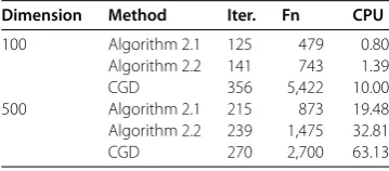
initial point is set asx=rand(n, ). Tables - give the numerical results by Algorithm .,
Algorithm ., and CGD with different dimensions, where Iter. denotes the iteration num-ber, Fn denotes the number of function evaluations, and CPU denotes the CPU time in seconds when the algorithms terminate.
Table 1 Numerical results with different dimensions of Problem 1
Dimension Method Iter. Fn CPU
1,000 Algorithm 2.1 1 5 0.02 Algorithm 2.2 1 5 0.02
CGD 11 51 0.03
5,000 Algorithm 2.1 1 5 0.03 Algorithm 2.2 1 5 0.03
CGD 12 56 0.16
50,000 Algorithm 2.1 1 5 0.14 Algorithm 2.2 1 5 0.11
CGD 13 60 1.33
100,000 Algorithm 2.1 1 5 0.25 Algorithm 2.2 1 5 0.25
[image:12.595.214.379.272.410.2]CGD 13 60 2.86
Table 2 Numerical results with different dimensions of Problem 2
Dimension Method Iter. Fn CPU
1,000 Algorithm 2.1 10 59 0.05 Algorithm 2.2 8 52 0.05
CGD 12 59 0.06
5,000 Algorithm 2.1 10 59 0.17 Algorithm 2.2 8 52 0.16
CGD 12 59 0.22
50,000 Algorithm 2.1 11 64 1.58 Algorithm 2.2 10 63 1.47
CGD 12 59 1.55
100,000 Algorithm 2.1 12 69 3.50 Algorithm 2.2 10 63 3.19
CGD 13 69 3.88
Table 3 Numerical results with different dimensions of Problem 3
Dimension Method Iter. Fn CPU
100 Algorithm 2.1 125 479 0.80
Algorithm 2.2 141 743 1.39
CGD 356 5,422 10.00
500 Algorithm 2.1 215 873 19.48
Algorithm 2.2 239 1,475 32.81
CGD 270 2,700 63.13
5 Conclusions
Two spectral gradient projection methods for solving constrained equations have been developed, which are not only derivative-free, but also completely matrix-free. Conse-quently, they can be applied to solve large-scale nonsmooth constrained equations. We established the global convergence without the requirement of differentiability of the equations, and presented the linear convergence rate under standard conditions. We also reported some numerical results to show the efficiency of the proposed methods.
Competing interests
The authors declare that they have no competing interests.
Authors? contributions
[image:12.595.207.387.447.526.2]Author details
1School of Mathematics and Statistics, Zhejiang University of Finance and Economics, Xueyuan Street, Hangzhou, 310018,
P.R. China.2School of Economics and Management, Tongji University, Siping Street, Shanghai, 200092, P.R. China.
Acknowledgements
The authors gratefully acknowledge the helpful comments and suggestions of the anonymous reviewers. This work is supported by the National Natural Science Foundation of China (71371139, 11302188), the Shanghai Shuguang Talent Project (13SG24), the Shanghai Pujiang Talent Project (12PJC069), and the Foundation of Teachers Professional Development of Zhejiang Provincial Visiting Scholar in Higher School.
Received: 20 July 2014 Accepted: 12 December 2014
References
1. Dirkse, SP, Ferris, MC: MCPLIB: a collection of nonlinear mixed complementarity problems. Optim. Methods Softw.5, 319-345 (1995)
2. Wood, AJ, Wollenberg, BF: Power Generation, Operation, and Control. Wiley, New York (1996)
3. Meintjes, K, Morgan, AP: A methodology for solving chemical equilibrium systems. Appl. Math. Comput.22, 333-361 (1987)
4. Qi, LQ, Tong, XJ, Li, DH: An active-set projected trust region algorithm for box constrained nonsmooth equations. J. Optim. Theory Appl.120, 601-625 (2004)
5. Ortega, JM, Rheinboldt, WC: Iterative Solution of Nonlinear Equations in Several Variables. Academic Press, New York (1970)
6. Yu, ZS, Lin, J, Sun, J, Xiao, YH, Liu, LY, Li, ZH: Spectral gradient projection method for monotone nonlinear equations with convex constraints. Appl. Numer. Math.59, 2416-2423 (2009)
7. Liu, SY, Huang, YY, Jiao, HW: Sufficient descent conjugate gradient methods for solving convex constrained nonlinear monotone equations. Abstr. Appl. Anal.2014, Article ID 305643 (2014)
8. Sun, M, Liu, J: Three derivative-free projection methods for large-scale nonlinear equations with convex constraints. J. Appl. Math. Comput. (2014). doi:10.1007/s12190-014-0774-5
9. Barzilai, J, Borwein, JM: Two point stepsize gradient methods. IMA J. Numer. Anal.8, 141-148 (1988)
10. Birgin, EG, Martinez, JM, Raydan, M: Spectral projected gradient methods: review and perspectives. J. Stat. Softw.60, 1-21 (2014)
11. Fletcher, R, Reeves, C: Function minimization by conjugate gradients. Comput. J.7, 149-154 (1964)
12. Dai, YH, Liao, LZ:R-Linear convergence of the Barzilai and Borwein gradient method. IMA J. Numer. Anal.22, 1-10 (2002)
13. Wang, CW, Wang, YJ, Xu, CL: A projection method for a system of nonlinear monotone equations with convex constraints. Math. Methods Oper. Res.66, 33-46 (2007)
14. Zheng, L: A new projection algorithm for solving a system of nonlinear equations with convex constraints. Bull. Korean Math. Soc.50, 823-832 (2013)