R E S E A R C H
Open Access
Stochastic inequalities and applications to
dynamics analysis of a novel SIVS epidemic
model with jumps
Xiaona Leng
1, Tao Feng
1and Xinzhu Meng
1,2**Correspondence: [email protected] 1College of Mathematics and Systems Science, Shandong University of Science and Technology, Qingdao, 266590, P.R. China
2State Key Laboratory of Mining Disaster Prevention and Control Co-founded by Shandong Province and the Ministry of Science and Technology, Shandong University of Science and Technology, Qingdao, 266590, P.R. China
Abstract
This paper proposes a new nonlinear stochastic SIVS epidemic model with double epidemic hypothesis and Lévy jumps. The main purpose of this paper is to investigate the threshold dynamics of the stochastic SIVS epidemic model. By using the
technique of a series of stochastic inequalities, we obtain sufficient conditions for the persistence in mean and extinction of the stochastic system and the threshold which governs the extinction and the spread of the epidemic diseases. Finally, this paper describes the results of numerical simulations investigating the dynamical effects of stochastic disturbance. Our results significantly improve and generalize the
corresponding results in recent literatures. The developed theoretical methods and stochastic inequalities technique can be used to investigate the high-dimensional nonlinear stochastic differential systems.
Keywords: stochastic SIVS epidemic model; Lévy jumps; persistence in mean; double epidemic diseases; Doob’s martingale inequality; Hölder’s inequality
1 Introduction
Mathematical inequalities are widely used in many fields of mathematical analysis, es-pecially differential systems [–]. Recently, the inequality technique was applied to stochastic differential systems [–], impulsive differential systems [–], and impul-sive stochastic differential systems [], thus some new results have been obtained.
As an important factor threatening the safety of human life and property, the investiga-tion of epidemic has received extensive atteninvestiga-tion from experts in various fields [–]. Generally speaking, medical researchers often use observation and experimental meth-ods to study the behavior of epidemics. Recently, however, a number of experts in the field of mathematics have also been interested in the study of epidemics. They have used mathematical methods to analyze the spread and control of epidemics [–]. Kermack and McKendrick’s pioneering work on the development of an epidemic disease is one of the typical examples. They established an SIS compartment model and proposed the fa-mous threshold theory, which has laid a solid foundation for the study of the dynamics of infectious diseases [].
The SIS model based on the deterministic ordinary differential equation is given by
⎧ ⎨ ⎩ ˙
S(t) =A–βS(t)I(t) –uS(t) +rI(t), ˙
I(t) =βS(t)I(t) – (u+α+r)I(t). ()
In system (),βS(t) represents the number of people infected by a patient within a unit time att. But in reality, the number of people who can be exposed to a patient at a time is limited. To this end, some authors have introduced a saturated infection rate to study the dynamic behavior of the disease [–]. In addition, all creatures on the earth are infected by a variety of environmental noises, of course, the disease is no exception. Motivated by this, some scholars have studied the infection system with environmental noises (such as Brownion noise, Markov noise and Lévy noise) [–]. Meanwhile, populations may be affected by different kinds of infectious diseases at the same time. Therefore, it is of great significance to study the epidemic model with multiple diseases [–].
Recently, Meng et al. [] considered a novel nonlinear stochastic SIS epidemic model with double epidemic hypothesis as follows:
⎧ ⎪ ⎪ ⎪ ⎪ ⎪ ⎨ ⎪ ⎪ ⎪ ⎪ ⎪ ⎩
dS= (A–uS(t) –βS(t)I(t)
a+I(t) –
βS(t)I(t)
a+I(t) +rI(t) +rI(t))dt
–σS(t)I(t)
a+I(t) dB(t) –
σS(t)I(t)
a+I(t) dB(t),
dI= (βaS+(tI)I(t()t)– (u+α+r)I(t))dt+σaS(+tI)I(t()t)dB(t),
dI= (βaS+(tI)I(t()t)– (u+α+r)I(t))dt+σaS(+tI)I(t()t)dB(t).
()
They obtained the threshold of system () for the extinction and the persistence in mean of the epidemic diseases. Based on system (), recently, Zhang et al. [] proposed an SIS system with double epidemic diseases driven by Lévy jumps as follows:
⎧ ⎪ ⎪ ⎪ ⎪ ⎪ ⎪ ⎪ ⎪ ⎪ ⎪ ⎪ ⎨ ⎪ ⎪ ⎪ ⎪ ⎪ ⎪ ⎪ ⎪ ⎪ ⎪ ⎪ ⎩
dS= (A–uS(t) –βS(t)I(t)
a+I(t) –
βS(t)I(t)
a+I(t) +rI(t) +rI(t))dt
+σS(t)dB(t) +
Zγ(u)S(t–)N(dt,du),
dI= (βaS+(tI)I(t()t)– (u+α+r)I(t))dt +σI(t)dB(t) +
Zγ(u)I(t–)N(dt,du),
dI= (βaS(+tI)I(t()t)– (u+α+r)I(t))dt +σI(t)dB(t) +
Zγ(u)I(t–)N(dt,du).
()
Motivated by the above works, in this paper, we propose a stochastic SIVS model with double epidemic diseases and Lévy jumps under vaccination as follows:
⎧ ⎪ ⎪ ⎪ ⎪ ⎪ ⎪ ⎪ ⎪ ⎪ ⎪ ⎪ ⎪ ⎪ ⎪ ⎪ ⎪ ⎪ ⎪ ⎪ ⎪ ⎨ ⎪ ⎪ ⎪ ⎪ ⎪ ⎪ ⎪ ⎪ ⎪ ⎪ ⎪ ⎪ ⎪ ⎪ ⎪ ⎪ ⎪ ⎪ ⎪ ⎪ ⎩
dS= (( –q)– (u+p)S(t) – βS(t)I(t)
α+I(t) –
βS(t)I(t)
α+I(t)
+rI(t) +rI(t) +δV(t))dt +σS dB(t) +
Zγ(u)S(t–)N(dt,du),
dI= (βαS+(tI)I(t()t)– (u+d+r)I(t))dt
+σIdB(t) +
Zγ(u)I(t–)N(dt,du),
dI= (βαS(+tI)I(t()t)– (u+d+r)I(t))dt
+σIdB(t) +
Zγ(u)I(t–)N(dt,du),
dV= [q+pS(t) – (u+δ)V(t)]dt+σV dB(t) +Zγ(u)V(t–)N(dt,du),
()
whereS(t),I(t),I(t),V(t), respectively, stand for the density of susceptible, infectiveA, infectiveBand vaccinated individuals at timet,is a constant input of new numbers into the population,qmeans a fraction of vaccinated for the newborn,βiis the infection rate
coefficient fromIi(t) (i= , ) toS(t), respectively.urepresents the natural death rate of
S(t),I(t),I(t),V(t),pis the proportional coefficient of vaccinated for the susceptible,ri,
diis the recovery rate and disease-caused death rate ofIi(t),i= , , respectively.δstands
for the rate of losing their immunity for vaccinated individuals,αandαare the so-called half-saturation constants, respectively.B(t) = (B(t),B(t),B(t),B(t)) is a standard Brow-nian motion with intensityσi> (i= , , , ).
Throughout this paper, let (,F,{F}t≥,P) be a complete probability space with a
fil-tration{Ft}t≥ satisfying the usual conditions (i.e. it is increasing and right continuous
while F contains all P-null sets). Function Bi(t) (i= , , , ) is a Brownian motion
defined on the complete probability space , the intensity ofBi(t) is σi (i= , , , ).
N(dt,du) =N(dt,du) –λ(du)dt,N is a Poisson counting measure on (, +∞)×Z,λis the characteristic measure ofNon a measurable subsetZ,λ(Z) < +∞,γi(i= , , , ) is
bounded and continuous with respect toλand isB(Z)×Ft-measurable. For an integrable
functionX(t) on [, +∞), we defineX(t)=ttX(s)ds.
2 Main results
The main purpose of this paper is to investigate the threshold dynamics of the stochas-tic SIVS epidemic model. In this section, by using the technique of a series of stochasstochas-tic inequalities, we obtain sufficient conditions for the persistence in mean and extinction of the stochastic system and the threshold which governs the extinction and the spread of epidemic diseases.
2.1 Preliminary knowledge
For the sake of notational simplicity, we define
bi=
σ
i +
Z
γi(u) –ln
+γi(u)
λ(du), i= , , , ;
Ri=
βi(u+δ–uq)
u+uδ+up –αi(u+di+ri+bi), i= , ; ˇ
γ(u) =maxγ(u),γ(u),γ(u),γ(u)
;
ˆ
γ(u) =minγ(u),γ(u),γ(u),γ(u)
;
φ=
Z +γˇ(u)
– –γˆ(u)v(du);
σ=max{σ,σ,σ,σ}.
Throughout this paper, suppose that the following two assumptions hold.
Assumption . The following hold:
(i) +γi(u) > ;
(ii) Z[γi(u) –ln( +γi(u))]λ(du) <∞,i= , , , ,u∈Z.
Remark . This assumption means that the intensities of Lévy noises are not infi-nite.
Assumption . Suppose that there exists some> such that the following inequality holds:
b=u––
σ
–φ
> .
Definition .([])
(i) The speciesX(t)is said to be extinctive iflimt→+∞X(t) = ;
(ii) The speciesX(t)is said to be persistent in mean iflimt→+∞X(t)∗> .
The following elementary inequality will be used frequently in the sequel.
Lemma .(Burkholder-Davis-Gundy inequality []) Let g∈L(R
+;Rd×m).For any t≥ ,define
x(t) =
t
g(s)dB(s), A(t) =
t
Then,for every p> ,there exist two positive constants cp,Cpsuch that
cpEA(t) p/
≤E sup
≤s≤t|x(s)|p
≤CpEA(t) p/
, t≥,
where cp,Cponly depend on p.
Lemma .(Chebyshev inequality []) For any c> ,p> ,X∈Lp, the following
in-equality holds:
Pw:X(w)≥c≤c–pE|X|p.
Lemma .(Hölder inequality []) For any ai,bi∈R and k≥,if p,q> andp+q= ,
the following inequality holds:
k
i=
aibi
≤
k
i= |ai|p
/pk
i= |bi|q
/q
.
Lemma .(Doob’s martingale inequality []) Let X be a submartingale taking nonneg-ative real values,either in discrete or continuous time.That is,for all times s and t with s<t,
Xs≤E[Xt|Fs].
Then,for any constant C> ,
P sup
≤t≤T
Xt≥C
≤E[|XT|]
C ,
where P denotes the probability measure on the sample spaceof the stochastic process X: [,T]×→[, +∞)and E denotes the expected value with respect to the probability measure P.
Lemma .([, ]) Assume that X(t)∈R+is an Itô’s-Lévy process of the form
dX(t) =FXt–,t–dt+GXt–,t–dB(t) +
ZH
Xt–,t–,uN(dt,du),
where F:Rn×R
+×S→Rn,G:Rn×R+×S→Rnand H:Rn×R+×S×Z→Rnare
measurable functions.
Given V∈C,(Rn×R
+×S;R+),we define the operator LV by
LV(X,t) =Vt(X,t) +VX(X,t)F(X,t) +
trace G
T(X,t)V
XX(X,t)G(X,t)
+
Z
VX+H(X,t)–V(X,t) –VX(X,t)H(X,t,u)
λ(du),
where
Vt(X,t) =
∂VX(X,t)
VX(X,t) =
∂VX(X,t)
∂X
, . . . ,∂VX(X,t)
∂Xn
,
VXX(X,t) =
∂VX(X,t)
∂Xi∂Xj
n×n
.
Then the generalized Itô’s formula with Lévy jumps is given by
dV(X,t) =LV(X,t)dt+VX(X,t)G(X,t)dB(t) +
Z
VX+H(X,t)–V(X,t)N(dt,du).
Lemma .([]) Let X(t)∈C(×[, +∞),R+).We have the following conclusions. (i) If there existT> ,λ> ,λ,m,nisuch that whent≥T,
lnX(t)≤λt–λ
t
X(s)ds+mB(t) +
j
i=
ni
t
Z
ln +γi(u)(ds,du) a.s.,
then
⎧ ⎨ ⎩
X∗≤ λ
λ a.s., ifλ≥;
limt→+∞X(t) = a.s., ifλ< .
(ii) If there existT> ,λ> ,λ> ,m,nisuch that whent≥T,
lnX(t)≥λt–λ
t
X(s)ds+mB(t) +
j
i=
ni
t
Z
ln +γi(u)(ds,du) a.s.,
thenX∗≥λλ a.s.
Lemma . For any initial value(S(),I(),I(),V())∈R+,the solution(S(t),I(t),I(t),
V(t))of model()has the following property:
lim
t→∞
S(t) +I(t) +I(t) +V(t)
t = a.s.
Moreover,
lim
t→∞
S(t)
t = , tlim→∞
I(t)
t = ,
lim
t→∞
I(t)
t = , tlim→∞
V(t)
t = a.s.
lim
t→∞
lnS(t)
t ≤, tlim→∞
lnI(t)
t ≤,
lim
t→∞
lnI(t)
t ≤, tlim→∞
lnV(t)
t ≤ a.s.
Proof Define
Applying the generalized Itô’s formula toQ(X), we have
dQ(X)≤LQdt+X–σIdB(t) +σIdB(t) +σS dB(t) +σV dB(t)
+X
Z +γˇ(u)
–γˆN(dt,du), ()
where
LQ≤X–(–uX–dI–dI) +
(– )
X
–σX+φX
≤X–
X–
u––
σ
–φ
X
.
Choose a positive constant> that satisfies
b=u––
σ
–φ
> .
For any constantksatisfyingk∈(,b), one has
dektQX(t)≤L ektQX(t)dt+ektX– σI(s)dB(s) +σI(s)dB(s) +σS(s)dB(s) +σV(s)dB(s)
+ektX
Z +γˇ(u)
–γˆN(dt,du).
Integrating from totand taking expectation on both sides of (), we have
EektQX(t)≤QX()+E
t
keksQX(s)+eksLQX(s)ds
.
Easily, one has
kektQX(t)+ektLQX(t)≤kektX(t) +ektX–(t) –bX(t) +X(t) ≤ekt sup
X∈R+
X–
–
b–k
X+X
+
:=ektH.
Therefore
EX≤X ()
ekt +
H k ≤X
() +H:=M. ()
By Lemma ., applying the Burkholder-Davis-Gundy inequality, integrating equation () from tot, and for an arbitrarily small positive constantδ, one has
E sup
kδ≤t≤(k+)δ
X(t)≤EX(kδ)+Y+Y
where
Y =E
sup
kδ≤t≤(k+)δ
kδtX–(s) –bX(s) +X(s)ds
≤cE
sup
kδ≤t≤(k+)δ
kδtX(s)ds
≤cE (k+)δ
kδ
X(s)ds
≤cδE
sup
kδ≤t≤(k+)δ
X(s)ds
, k= , , . . .
and
Y =E
sup
kδ≤t≤(k+)δ
t
kδ
X–(s) σI(s)dB(s) +σI(s)dB(s) +σS(s)dB(s)
+σV(s)dB(s)
+
t
kδ
X(s)
Z +γˇ(u)
–γˆN(dt,du)
≤CE (k+)δ
kδ
X(–)σI+σI+σS+σVds
+CE (k+)δ
kδ
X
Z +γˇ(u)
–γˆ(u)v(du)ds
≤Cδ
σ+
Z +ˇ
γ(u)–γˆ(u)v(du)
E sup
kδ≤t≤(k+)δ
X
, k= , , . . . ,
wherec,C> .
So we have
E sup
kδ≤t≤(k+)δ
X(t)≤EX(kδ)+cδE
sup
kδ≤t≤(k+)δ
X(s)ds
+Cδ
σ+
Z +γˇ(u)
–γˆ(u)v(du)
×E sup
kδ≤t≤(k+)δ
X
.
Choose a positive constantδthat satisfies
cδ+Cδ
σ+
Z + ˇ
γ(u)–γˆ(u)v(du)
≤ .
Combining it with equation (), one has
E sup
kδ≤t≤(k+)δ
X(t)≤EX(kδ)≤M.
Applying the arbitrariness ofκX> and Lemma . for Chebyshev’s inequality, one
ob-tains
P sup
kδ≤t≤(k+)δ
X(t) > (kδ)+κX
≤E[supkδ≤t≤(k+)δX(t)]
(kδ)+κX
≤ M
Applying the Borel-Cantelli lemma [], for almost allω∈, one has
sup
kδ≤t≤(k+)δ
X(t)≤(kδ)+κX ()
holds for all but finitely manyk. Therefore, for any positive constantk≥kand almost all
ω∈, there isk(ω) such that equation () holds.
Thus, for almost allω∈, once conditionsk≥kandkδ≤t≤(k+ )δhold, then we have
lnX(t)
lnt ≤
( +κX)ln(kδ)
ln(kδ) = +κX. ()
Taking the limit superior on both sides of equation () and applying the arbitrariness of
κX> , one has
lim sup
t→∞
lnX(t)
lnt ≤ a.s.
Easily, for anysatisfying << +(uσ–φ), one hasu>
– σ
+φ. Therefore
lim sup
t→∞
lnX(t)
lnt ≤
a.s.
That is to say, for any constantτ satisfying <τ< –, there is a constantN=N(ω), and once conditiont≥Nholds, then we have
lnX(t)≤
+τ
lnt.
Therefore
lim
t→∞
X(t)
t =tlim→∞
S(t) +I(t) +I(t) +V(t)
t = ≤lim supt→∞
t+τ
t = a.s.
So
lim
t→∞
S(t)
t = , tlim→∞
I(t)
t = ,
lim
t→∞
I(t)
t = , tlim→∞
V(t)
t = a.s.
and
lim
t→∞
lnS(t)
t ≤, tlim→∞
lnI(t)
t ≤,
lim
t→∞
lnI(t)
t ≤, tlim→∞
lnV(t)
t ≤ a.s.
Lemma . For any initial value(S(),I(),I(),V())∈R+,the solution(S(t),I(t),I(t),
V(t))of model()has the following property:
lim
t→∞
t
I(s)dB(s)
t = , tlim→∞
t
Zγ(u)I(s)N(ds,du)
t = a.s.,
lim
t→∞
t
I(s)dB(s)
t = , tlim→∞
t
Zγ(u)I(s)N(ds,du)
t = a.s.,
lim
t→∞
t
S(s)dB(s)
t = , tlim→∞
t
Zγ(u)S(s)N(ds,du)
t = a.s.,
lim
t→∞
t
V(s)dB(s)
t = , tlim→∞
t
Zγ(u)V(s)N(ds,du)
t = a.s.
Proof Define
X(t) =
t
I(s)dB(s), Y(t) =
t
Zγ(u)I(s)
N(ds,du),
X(t) =
t
I(s)dB(s), Y(t) =
t
Z
γ(u)I(s)N(ds,du),
X(t) =
t
S(s)dB(s), Y(t) =
t
Zγ(u)S(s)
N(ds,du),
X(t) =
t
V(s)dB(s), Y(t) =
t
Zγ(u)V(s)
N(ds,du).
Applying Lemma . for the Burkholder-Davis-Gundy inequality and Lemma . for Hölder’s inequality, one has
Esup
≤s≤t
X(s)
≤CE
t
I(θ)dθ
≤CE
t
I(θ)dθ
,
Esup
≤s≤t
Y(s)
≤CE
t
ZI
(θ)γ(u)dθ
≤C Zγ
(u)v(du)
E
t
I(θ)dθ
for << +(uσ–φ). HereC= [ +
(–)–]
> is a constant.
Applying equation (), we have
E sup
k≤t≤(k+) X(s)
≤MC(k+ )
≤+
MCk
.
For any constantκX> , applying Lemma . for Doob’s martingale inequality, one
ob-tains
Pω: sup
k≤t≤(k+) X(t)
>k+κX+
≤E[supk≤t≤(k+)|X(k+ )|]
k+κX+ ≤
+MC k
k+κX+
≤+
MC
Applying the Borel-Cantelli lemma, one has
ln|X(t)|
lnt ≤
( +κX+
)lnk
lnk = +κX+
. ()
Taking the limit superior on both sides of equation () and applying the arbitrariness of
κX> , one has
lim sup
t→∞
ln|X(t)|
lnt ≤
+
a.s.
That is to say, for any constantτ satisfying <τ<–, there is a constantN=N(ω), and oncet≥N,w∈τ holds, then we have
lnX(t)≤
+
+τ
lnt. ()
Dividing both sides of equation () bytand taking the limit superior, we have
lim sup
t→∞ |X(t)|
t ≤lim supt→∞
t++τ
t = .
Combining it withlim inft→∞|Xt(t)|≥, one has
lim
t→∞
|X(t)|
t =tlim→∞
X(t)
t = a.s.
Similarly, one obtains
lim
t→∞
lnX(t)
t = , tlim→∞
lnX(t)
t = ,
lim
t→∞
lnX(t)
t = , tlim→∞
lnY(t)
t = ,
lim
t→∞
lnY(t)
t = , tlim→∞
lnY(t)
t = , tlim→∞
lnY(t)
t = .
This completes the proof.
Lemma . For any initial value(S(),I(),I(t),V())∈R+,model()has a unique
pos-itive solution(S(t),I(t),I(t),V(t))∈R+on t≥with probability.
Proof The proof is similar to Refs. [, ] by definingQ(S,I,I,V) =S– –lnS+I– –
lnI+I– –lnI+V– –lnV, and hence is omitted.
2.2 Stochastic disease-free dynamics
Theorem . Suppose that conditions R< and R< hold.Then,for any initial value (S(),I(),I(),V())∈R+,the solution(S(t),I(t),I(t),V(t))of model()has the
follow-ing property:
lim
t→∞Ii(t) = , i= , , tlim→∞
S(t) =(u+δ–uq)
lim
t→∞
V(t) = (p+uq)
u+uδ+up.
That is to say,the two epidemic diseases go to extinct almost surely.
Proof By equation (), one has
d
S+I+I+
δ u+δV
=(u+δ–uq)
u+δ –
u+uδ+up
u+δ S–
i=
(u+di)Ii
+σS dB(t) +
Zγ(u)S
t–N(dt,du)
+
i=
σiIidBi(t) +
Zγi(u)Ii
t–N(dt,du)
+ δ
u+δ
σV dB(t) +
Zγ(u)V
t–N(dt,du)
. ()
Dividing both sides of equation () bytand integrating over the time interval totyield
S(t) = u+δ
u+uδ+up !
(u+δ–uq) u+δ –
i= (u+di)
Ii(t) –(t)
"
, ()
where
(t) =
t
#
S(t) –S() +
i=
Ii(t) –Ii()
+ δ
u+δ
V(t) –V()
–
i=
t
σiIidBi(s) +
Zγi(u)Ii(s)
N(dt,du)
–
t
σS dB(s) +
Zγ(u)S(s)
N(dt,du)
– δ
u+δ
t
σV dB(s) +
Zγ(u)V(s)
N(dt,du) $
.
Applying Lemmas . and ., we obtain that
lim
t→+∞(t) = a.s. ()
Applying the generalized Itô’s formula in Lemma . toαlnI(t) +I(t) yields
d αlnI(t) +I(t)
= βS– (u+d+r)I–α(u+d+r) –αb
dt
+ (α+I)σdB(t) +
Z αln
+γ(u)
Dividing both sides of equation () by t, integrating over the time interval to tand taking the limit, one obtains that
αlnI(t) +I(t)
t =
αlnI() +I()
t +β
S(t) – (u+d+r)
I(t)
–α(u+d+r) –αb+
t
t
α+I(s)
σdB(s)
+
t
t
Z α
ln +γ(u)
+I(s)γ(u)N(dt,du). ()
Combining equations () and (), one obtains
αlnI(t)
t =
β(u+δ–uq)
u+uδ+up –α(u+d+r+b) –
β(u+δ)(u+d)
u+uδ+up
I(t)
–
β(u+δ)(u+d)
u+uδ+up + (u+d+r)
I(t) +
αlnI() +I()
t
–I(t)
t –
β(u+δ)
u+uδ+up(t) +
t
t
α+I(s)
σdB(s)
+
t
t
Z α
ln +γ(u)
+I(s)γ(u)N(dt,du)
=β(u+δ–uq)
u+uδ+up –α(u+d+r+b) –
β(u+δ)(u+d)
u+uδ+up
I(t)
–
β(u+δ)(u+d)
u+uδ+up + (u+d+r)
I(t) +(t), ()
where
(t) =
αlnI() +I()
t – I(t)
t –
β(u+δ)
u+uδ+up(t)
+
t
t
α+I(s)
σdB(s)
+
t
t
Z αln
+γ(u)
+I(s)γ(u)N(dt,du).
Similarly, applying the generalized Itô’s formula in Lemma . toαlnI(t) +I(t) yields
αlnI(t)
t =
β(u+δ–uq)
u+uδ+up –α(u+d+r+b) –
β(u+δ)(u+d)
u+uδ+up
I(t)
–
β(u+δ)(u+d)
u+uδ+up + (u+d+r)
I(t) +(t), ()
where
(t) =
αlnI() +I()
t – I(t)
t –
β(u+δ)
u+uδ+up(t)
+
t
t
α+I(s)
σdB(s)
+ t t Z αln
+γ(u)
Applying Lemmas . and ., we obtain that
lim
t→+∞i(t) = , i= , a.s. ()
By taking the limit superior of both sides of equation () and equation (), respectively, one has
lim sup
t→∞
αlnI(t)
t ≤
β(u+δ–uq)
u+uδ+up –α(u+d+r+b) =R< ,
lim sup
t→∞
αlnI(t)
t ≤
β(u+δ–uq)
u+uδ+up –α(u+d+r+b) =R< .
That is to say,
lim
t→∞Ii(t) = , i= , a.s. ()
Applying () and () into equation (), we obtain that
lim
t→∞
S(t) = u+δ
u+uδ+up !
(u+δ–uq) u+δ –
i=
(u+di)lim t→∞
Ii(t) – lim t→∞(t)
"
=(u+δ–uq)
u+uδ+up. ()
By equation (), one has
d(S+I+I+V) = –uS–uV– (u+d)I– (u+d)I
dt
+
i=
σiIidBi(t) +
Z γi(u)Ii
t–N(dt,du)
+σS dB(t) +
Zγ(u)S
t–N(dt,du)
+σV dB(t) +
Z γ(u)V
t–N(dt,du). ()
Dividing both sides of equation () byt, integrating over the time intervalt= totand taking the limit, one obtains that
lim
t→∞
V(t) =
u –tlim→∞
S(t) –
i=
u+di
u tlim→∞
Ii(t)
–lim
t→∞
S(t) –S() +%i=(Ii(t) –Ii()) +V(t) –V()
ut
+
utlim→∞
t
t
#
i=
σiIi(s)dBi(s) +
Z γ(u)I
s–N(ds,du)
+σS(s)dB(s) +
Zγ(u)S
s–N(ds,du)
+σV(s)dB(s) +
Z γ(u)V
s–N(ds,du) $
Applying (), (), Lemmas . and ., we have
lim
t→∞
V(t) =
u –
(u+δ–uq) u+uδ+up =
(p+uq) u+uδ+up.
This completes the proof.
2.3 Stochastic endemic dynamics
Theorem . For any initial value(S(),I(),I(),V())∈R+,the solution(S(t),I(t),
I(t),V(t))of model()has the following property:
(i) IfR> andR< ,then the epidemic diseaseI(t)is persistent in mean andI(t)
goes extinct,i.e.limt→∞I(t)=ϒR > ,limt→∞I(t) = a.s.Moreover,
lim
t→∞
S(t) =(u+δ–uq)
u+uδ+up –
(u+δ)(u+d)
u+uδ+up
R
ϒ
a.s.,
lim
t→∞
V(t) = (p+uq)
u+uδ+up–
(u+d)p
u(u+δ+p)
R
ϒ
a.s.
(ii) IfR< andR> ,then the epidemic diseaseI(t)goes extinct andI(t)is persistent
in mean,i.e.limt→∞I(t)= ,limt→∞I(t) = ϒR > a.s.Moreover,
lim
t→∞
S(t) =(u+δ–uq)
u+uδ+up –
(u+δ)(u+d)
u+uδ+up
R
ϒ
a.s.,
lim
t→∞
V(t) = (p+uq)
u+uδ+up–
(u+d)p
u(u+δ+p)
R
ϒ
a.s.
Proof Case (i): From equation () we have
αlnI(t)
t =
β(u+δ–uq)
u+uδ+up –α(u+d+r+b)
–
β(u+δ)(u+d)
u+uδ+up + (u+d+r)
I(t)
–β(u+δ)(u+d)
u+uδ+up
I(t) +(t)
=R–ϒ
I(t) –ϒ
I(t) +(t), ()
where
ϒ=
β(u+δ)(u+d)
u+uδ+up + (u+d+r), ϒ=
β(u+δ)(u+d)
u+uδ+up .
From Theorem ., whenR< one has
lim
t→∞I(t) = a.s. ()
Therefore, there exists an arbitrarily small constantε> such that whentis large enough, we haveI(t) <ε. Applying this into equation () leads to
R–ϒ
I(t) +(t)≥
αlnI(t)
t ≥R–ϒ
Applying Lemma . and the arbitrariness ofε, we obtain
lim
t→∞
I(t) =
R
ϒ
a.s. ()
Applying (), () and () into equation (), we obtain that
lim
t→∞
S(t) = u+δ
u+uδ+up !
(u+δ–uq) u+δ –
i=
(u+di)lim t→∞
Ii(t) – lim t→∞(t)
"
=(u+δ–uq)
u+uδ+up –
(u+δ)(u+d)
u+uδ+up
R
ϒ
. ()
Applying (), (), (), Lemmas . and . into equation (), we have
lim
t→∞
V(t) =
u –
(u+δ–uq) u+uδ+up +
(u+δ)(u+d)
u+uδ+up
R
ϒ
–u+d
u R
ϒ
= (p+uq)
u+uδ+up–
(u+d)p
u(u+δ+p)
R
ϒ .
Case (ii): From equation () we have
αlnI(t)
t =
β(u+δ–uq)
u+uδ+up –α(u+d+r+b) –
β(u+δ)(u+d)
u+uδ+up
I(t)
–
β(u+δ)(u+d)
u+uδ+up + (u+d+r)
I(t) +(t)
=R–ϒ
I(t) –ϒ
I(t) +(t), ()
where
ϒ=
β(u+δ)(u+d)
u+uδ+up , ϒ=
β(u+δ)(u+d)
u+uδ+up + (u+d+r).
From Theorem ., whenR< one has
lim
t→∞I(t) = a.s. ()
Therefore, there exists an arbitrarily small constantε> such that whentis large enough, we haveI(t) <ε. Applying this into equation () leads to
R–ϒ
I(t) +(t)≥
αlnI(t)
t ≥R–ϒ
I(t) –ϒε+(t).
Applying Lemma . and the arbitrariness ofε, we obtain
lim
t→∞
I(t) =
R
ϒ
Applying equations (), (), () into equation (), we obtain that
lim
t→∞
S(t) = u+δ
u+uδ+up !
(u+δ–uq) u+δ –
i=
(u+di)lim t→∞
Ii(t) – lim t→∞(t)
"
=(u+δ–uq)
u+uδ+up –
(u+δ)(u+d)
u+uδ+up
R
ϒ
. ()
Applying (), (), (), Lemmas . and . into equation (), we have
lim
t→∞
V(t) =
u –
(u+δ–uq) u+uδ+up +
(u+δ)(u+d)
u+uδ+up
R
ϒ
–u+d
u R
ϒ
= (p+uq)
u+uδ+up–
(u+d)p
u(u+δ+p)
R
ϒ .
This completes the proof.
Theorem . Suppose that conditions R> and R> hold.Let(S(t),I(t),I(t),V(t))be
the solution of model()with the initial value(S(),I(),I(),V())∈R+.
(i) IfϒR<ϒR,then the epidemic diseaseI(t)is persistent in mean andI(t)goes
extinct,i.e.limt→∞I(t)=ϒR > ,limt→∞I(t) = a.s.Moreover,
lim
t→∞
S(t) =(u+δ–uq)
u+uδ+up –
(u+δ)(u+d)
u+uδ+up
R ϒ a.s., lim t→∞
V(t) = (p+uq)
u+uδ+up–
(u+d)p
u(u+δ+p)
R
ϒ
a.s.
(ii) IfϒR<ϒR,then the epidemic diseaseI(t)goes extinct andI(t)is persistent in
mean,i.e.limt→∞I(t)= ,limt→∞I(t) = ϒR > a.s.Moreover,
lim
t→∞
S(t) =(u+δ–uq)
u+uδ+up –
(u+δ)(u+d)
u+uδ+up
R ϒ a.s., lim t→∞
V(t) = (p+uq)
u+uδ+up–
(u+d)p
u(u+δ+p)
R
ϒ
a.s.
(iii) IfϒR>ϒR,ϒR>ϒR,then the epidemic diseasesIandIare persistent
in mean.Moreover,
lim
t→∞
I(t) =
ϒR–ϒR
ϒϒ–ϒϒ
, lim
t→∞
I(t) =
ϒR–ϒR
ϒϒ–ϒϒ
a.s.,
lim
t→∞
S(t) =(u+δ–uq)
u+uδ+up –
(u+δ)(u+d)
u+uδ+up
ϒR–ϒR
ϒϒ–ϒϒ
–(u+δ)(u+d)
u+uδ+up
ϒR–ϒR
ϒϒ–ϒϒ
a.s.,
lim
t→∞
V(t) = (p+uq)
u+uδ+up–
(u+d)p
u(u+δ+p)
ϒR–ϒR
ϒϒ–ϒϒ
– (u+d)
u(u+δ+p)
ϒR–ϒR
ϒϒ–ϒϒ
Proof Case (i): Note that
lim sup
t→+∞
lnI(t)
t ≤,
there exists an arbitrarily small constantε> such that whentis large enough, we have
lnI(t)
t <ε.
From equation () and equation (), whentis large enough, one has
ϒαlnI(t)
t =ϒR–ϒR– (ϒϒ–ϒϒ)
I(t) +ϒα
lnI(t)
t
+ϒ(t) –ϒ(t)
≤ϒR–ϒR– (ϒϒ–ϒϒ)
I(t) +ϒαε
+ϒ(t) –ϒ(t). ()
SinceϒR<ϒRandϒϒ>ϒϒ, taking the limit superior of both sides of equa-tion (), applying equaequa-tion () and the arbitrariness ofε, we have
lim sup
t→+∞
lnI(t)
t ≤
ϒR–ϒR
ϒα
< .
That is to say,
lim
t→∞I(t) = a.s.
By using the method of Case (ii) in Theorem ., one obtains the persistence in mean of
I(t),S(t) andV(t), and hence is omitted.
Case (ii): The proof of Case (ii) is similar to the proof of Case (i) in this subsection and hence is omitted.
Case (iii): SinceϒR>ϒRandϒϒ>ϒϒ, using Lemma . and the arbitrari-ness ofεfor equation (), one obtains that
lim sup
t→+∞
I(t) ≤
ϒR–ϒR
ϒϒ–ϒϒ
a.s. ()
Similarly, whenϒR>ϒR, we have
lim sup
t→+∞
I(t) ≤
ϒR–ϒR
ϒϒ–ϒϒ
a.s. ()
From equation (), there exists an arbitrarily small constantε> such that whentis large enough, we have
I(t) ≤
ϒR–ϒR
ϒϒ–ϒϒ
Applying equation () into equation (), one obtains that
αlnI(t)
t =R–ϒ
I(t) –ϒ
I(t) +(t)
≥R–ϒ
I(t) –ϒε–ϒ
ϒR–ϒR
ϒϒ–ϒϒ
+(t).
By using Lemma . and the arbitrariness ofε, we obtain that
lim inf
t→+∞
I(t) ≥
ϒR–ϒR
ϒϒ–ϒϒ
a.s. ()
Similarly, one obtains
lim inf
t→+∞
I(t) ≥
ϒR–ϒR
ϒϒ–ϒϒ
a.s. ()
Applying equations (), (), () and () leads to
lim
t→+∞
I(t) =
ϒR–ϒR
ϒϒ–ϒϒ
, lim
t→+∞
I(t) =
ϒR–ϒR
ϒϒ–ϒϒ
a.s. ()
Applying () and () into equation (), we obtain that
lim
t→∞
S(t) = u+δ
u+uδ+up !
(u+δ–uq) u+δ –
i=
(u+di)lim t→∞
Ii(t) – lim t→∞(t)
"
=(u+δ–uq)
u+uδ+up –
(u+δ)(u+d)
u+uδ+up
ϒR–ϒR
ϒϒ–ϒϒ
–(u+δ)(u+d)
u+uδ+up
ϒR–ϒR
ϒϒ–ϒϒ
. ()
Applying (), (), Lemmas . and . into equation (), we have
lim
t→∞
V(t) =
u –
(u+δ–uq) u+uδ+up +
(u+δ)(u+d)
u+uδ+up
ϒR–ϒR
ϒϒ–ϒϒ
–u+d
u
ϒR–ϒR
ϒϒ–ϒϒ
+(u+δ)(u+d)
u+uδ+up
ϒR–ϒR
ϒϒ–ϒϒ
–u+d
u
ϒR–ϒR
ϒϒ–ϒϒ
= (p+uq)
u+uδ+up–
(u+d)p
u(u+δ+p)
ϒR–ϒR
ϒϒ–ϒϒ
– (u+d)p
u(u+δ+p)
ϒR–ϒR
ϒϒ–ϒϒ .
This completes the proof.
3 Conclusions and numerical simulations
persistence in mean and extinction of the two diseases. Compared with the existing work in Refs. [] and [], the model constructed in this paper also considers the efficiency of vaccination. When all the coefficients related to the vaccination are , system () is similar to systems () and () in Refs. [] and [], in addition, our conclusion is consistent with them. That is to say, systems () and () in Refs. [] and [] are a special case of our system (). The theoretical results of this article can be used as a reference for the control of infectious diseases.
To sum up, we have the following conclusions:
I. Stochastic disease-free dynamics WhenR< andR< hold, we have
lim
t→∞Ii(t) = , i= , , tlim→∞
S(t) =(u+δ–uq)
u+uδ+up,
lim
t→∞
V(t) = (p+uq)
u+uδ+up.
That is to say, the two epidemic diseases go to extinct almost surely. II. Stochastic endemic dynamics
(i) If one of the following conditions holds: • R> ,R< ,
• R,R> ,ϒR<ϒR, then we have
lim
t→∞
I(t) =
R
ϒ
> , lim
t→∞I(t) = a.s.,
lim
t→∞
S(t) =(u+δ–uq)
u+uδ+up –
(u+δ)(u+d)
u+uδ+up
R
ϒ a.s.,
lim
t→∞
V(t) = (p+uq)
u+uδ+up–
(u+d)p
u(u+δ+p)
R
ϒ a.s.
That is to say, the epidemic diseaseI(t)is persistent in mean andI(t)is extinct. (ii) If one of the following conditions hold:
• R< ,R> ,
• R,R> ,ϒR<ϒR, then we have
lim
t→∞
I(t) = , lim
t→∞I(t) =
R
ϒ
> a.s.,
lim
t→∞
S(t) =(u+δ–uq)
u+uδ+up –
(u+δ)(u+d)
u+uδ+up
R
ϒ a.s.,
lim
t→∞
V(t) = (p+uq)
u+uδ+up–
(u+d)p
u(u+δ+p)
R
ϒ a.s.
That is to say, the epidemic diseaseI(t)is extinct andI(t)is persistent in mean. (iii) IfϒR>ϒR,ϒR>ϒRhold, then we have
lim
t→∞
I(t) =
ϒR–ϒR
ϒϒ–ϒϒ
, lim
t→∞
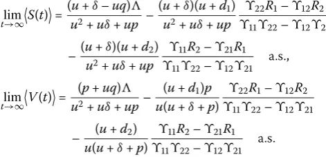
I(t) =
ϒR–ϒR