Convergence analysis of a variable metric forward–backward splitting algorithm with applications

(1)

R E S E A R C H

Open Access

Convergence analysis of a variable metric

forward–backward splitting algorithm with

applications

Fuying Cui

1

_{, Yuchao Tang}

1,2*

_{and Chuanxi Zhu}

1,2

*_{Correspondence:}

[email protected]

1_{Department of Mathematics,}

Nanchang University, Nanchang, P.R. China

2_{School of Management, Nanchang}

University, Nanchang, P.R. China

Abstract

The forward–backward splitting algorithm is a popular operator-splitting method for solving monotone inclusion of the sum of a maximal monotone operator and an inverse strongly monotone operator. In this paper, we present a new convergence analysis of a variable metric forward–backward splitting algorithm with extended relaxation parameters in real Hilbert spaces. We prove that this algorithm is weakly convergent when certain weak conditions are imposed upon the relaxation

parameters. Consequently, we recover the forward–backward splitting algorithm with variable step sizes. As an application, we obtain a variable metric forward–backward splitting algorithm for solving the minimization problem of the sum of two convex functions, where one of them is diﬀerentiable with a Lipschitz continuous gradient. Furthermore, we discuss the applications of this algorithm to the fundamental of the variational inequalities problem, constrained convex minimization problem, and split feasibility problem. Numerical experimental results on LASSO problem in statistical learning demonstrate the eﬀectiveness of the proposed iterative algorithm.

MSC: 90C25; 47H05; 65K05

Keywords: Forward–backward splitting algorithm; Monotone inclusion; Variable metric; Split feasibility problem

1 Introduction

LetHbe a real Hilbert space with inner product·,·and induced norm·. The forward– backward splitting algorithm is a classical operator-splitting algorithm, which solves the monotone inclusion problem

ﬁndx∈Hsuch that 0∈Ax+Bx, (1.1)

whereA:H→2H_{is a maximal monotone operator and}_B_:_H_→_H_{is a}_β_{-inverse strongly}

monotone operator (see Sect.2for the precise deﬁnition) for someβ> 0. The forward– backward splitting algorithm, which dates back to the original work of Lions and Mercier [1], has been studied and reported extensively in the literature; see, for example, [2–6]. The emergence of compressive sensing theory and large-scale optimization problems as-sociated with signal and image processing has resulted in the forward–backward splitting

(2)

algorithm receiving much attention in recent years. A forward–backward splitting algo-rithm with relaxation and errors in Hilbert spaces was proposed by Combettes [4]. More precisely, letx0∈H, set

xk+1=xk+λk

JγkA

xk–γk(Bxk+bk)

+ak–xk

, k≥0, (1.2)

where{γk} ⊂(0, 2β),{λk} ⊂(0, 1],{ak}and{bk}are absolutely summable sequences inH. In addition,JγkA:= (I+γkA)

–1_{denotes the resolvent of operator}_A_{with index}_γ

k> 0.

Com-bettes [4] proved the convergence of the iterative scheme (1.2) when certain conditions are imposed upon the parameters. Jiao and Wang [7] proved the convergence of (1.2) by requiring the parameters{λk}such that{λk} ⊂(0,₂_β4₊β_γ

k) whenbk= 0. It is easy to see that

4β

2β+γk is strictly larger than one when{γk} ⊂(0, 2β). Further, Combettes and Yamada [8] improved the range of the relaxation parameters{λk}in (1.2) to (0,4β–γk

2β ). After a

sim-ple calculation, we know that 4β–γk

2β > 4β

2β+γk. Therefore, the range of{λk}in the work of Combettes and Yamada [8] is larger than that of Jiao and Wang [7].

In the case when γk=γ andak=bk= 0, the iterative scheme (1.2) is reduced to the

forward–backward splitting algorithm with a constant step size [9]:

xk+1=xk+λk

JγA(xk–γBxk) –xk

, k≥0, (1.3)

whereγ ∈(0, 2β) and{λk} ⊂(0,4β₂–_βγ). Bauschke and Combettes [9] obtained the conver-gence of the iterative algorithm (1.3) by adopting the Krasnosekii–Mann (KM) iteration for computing the ﬁxed points of nonexpansive operators. Some recent progress on the KM iteration for solving ﬁxed point problem and split inclusion problem can be found in [10–12]. The forward–backward splitting algorithm with constant step size (1.3) is usu-ally considered to be stationary, whereas the forward–backward splitting algorithm with variable step sizes (1.2) is referred to as non-stationary.

It is worth mentioning that by lettingλk= 1, then (1.3) reduces to the classical forward–

backward splitting algorithm. More precisely, the iterative sequence{xk}is deﬁned by

xk+1=JγA(xk–γBxk), k≥0. (1.4)

In the context of convex optimization, the forward–backward splitting algorithm is equiv-alent to the so-called proximal gradient algorithm (PGA) applied to solve the following convex minimization problem:

min

x∈Hf(x) +g(x), (1.5)

where f :H→R is convex, diﬀerentiable with anL-Lipschitz continuous gradient for someL> 0 andg:H→(–∞, +∞] is a proper, lower semicontinuous, convex function. The convex optimization problem (1.5) has found widespread application in signal and image processing, for example, [13–17]. As a consequence of [4], Combettes and Wajs [18] employed the forward–backward splitting algorithm (1.2) to solve the minimization problem (1.5). The obtained iterative algorithm is deﬁned as

xk+1=xk+λk

prox_γ

kg

xk–γk

∇f(xk) +bk

+ak–xk

(3)

where{γk} ⊂(0, 2/L),{λk} ⊂(0, 1], and{ak},{bk}are absolutely summable sequences inH.

prox_γ_g denotes the proximity operator ofgwith indexγ > 0. In addition, Combettes and Wajs [18] presented applications of this algorithm to many concrete convex optimization problems. This iterative algorithm (1.6) was subsequently improved by Combettes and Yamada [8] who extended the range of the relaxation parameters{λk}.

Inspired by solving large-scale convex optimization problems arising in image process-ing, machine learnprocess-ing, and economic management, many efficient primal–dual splitting algorithms have been proposed for structured monotone inclusions involving maximal monotone operators and single-valued Lipschitz or inverse strongly monotone opera-tors; see, for example, [19, 20]. Although these monotone inclusions are more compli-cated than the monotone inclusion problem (1.1), they can be transformed into the form of this problem in a suitable product space. Therefore, it is natural to consider using the forward–backward splitting algorithm (e.g., (1.2) or (1.3)) to solve the equivalent mono-tone inclusion problem. Because the backward steps cannot be decomposed, direct use of the forward–backward splitting algorithm often fails to obtain a completely splitting algorithm. Many researchers attempted to overcome this difficulty by investigating vari-able metric operator splitting algorithms. The use of a suitvari-able varivari-able metric envari-ables the implicit step of backward splitting to be easily decomposed. For example, the primal– dual hybrid gradient algorithm [21] (also known as the primal–dual of the Chambolle– Pock algorithm [22]) is equivalent to the variable metric proximal point algorithm [23, 24]. We refer the readers to a subsequent paper [25] for more details. V˜u [26] proposed a variable metric extension of the forward–backward–forward splitting algorithm [3] for solving monotone inclusion of the sum of a maximal monotone operator and a monotone Lipschitzian operator in Hilbert spaces. Liang [27] proposed a variable metric multi-step inertial operator-splitting algorithm for solving the monotone inclusion problem (1.1). Bonettini et al. [28] developed a scaled inertial forward–backward splitting algorithm for solving (1.1) in the context of convex minimization. Neither of the respective algorithms in the work by Liang [27] and Bonettini et al. [28] was compatible with the relaxation strat-egy. The variable metric forward–backward splitting algorithm was originally studied in finite-dimensional Hilbert spaces [2,29]; however, the methods in these studies either had to be strongly monotone to study the convergence rate or they did not make use of the in-verse strongly monotone property ofBin (1.1). For infinite-dimensional Hilbert spaces, Combettes and V˜u [30] proposed a variable metric forward–backward splitting algorithm to solve (1.1) and analyzed its weak and strong convergence. This algorithm is defined as follows. Letx0∈H, and set

⎧ ⎨ ⎩

yk=xk–γkUk(Bxk+bk),

xk+1=xk+λk(JγkUkA(yk) +ak–xk),

(1.7)

where{Uk} ⊂Pα(H),{λk} ⊂(0, 1],{γk} ⊂(0, 2β),{ak}and{bk}are absolutely summable

sequences inH. This algorithm (1.7) includes a variable metric, variable step sizes, relax-ation parameter, and errors. It includes nearly all of the forward–backward type of split-ting algorithms mentioned above. For example, by letsplit-tingUk=Iin (1.7), it is reduced to

(4)

forward–backward splitting algorithm by replacing the relaxation parameters{λk}in (1.7) with self-adjoint, strong positive linear operators. However, this approach still requires the maximum eigenvalue of the operators to be smaller than one.

The purpose of this paper is to introduce a new convergence analysis for the variable metric forward–backward splitting algorithm (1.7) with an extended range of relaxation parameters. We prove the weak convergence of the variable metric forward–backward splitting algorithm by setting the relaxation parameter{λk}larger than one in real Hilbert spaces. To achieve this goal, we make full use of the averaged and firmly nonexpansive property of operatorsJγkUkA(I–γkUkB) andJγkUkA, whereλk> 0 andUk∈Pα(H). In con-trast, existing solutions mainly rely onJγkUkAbeing firmly nonexpansive. Consequently, we obtain the convergence of the forward–backward splitting algorithm with variable step sizes. Moreover, we impose a slightly weak condition on the relaxation parameters to ensure the convergence of this algorithm. The results we obtained complement and extend those of Combettes and Yamada [8]. As an application, we obtain the variable met-ric forward–backward splitting algorithm for solving the minimization problem (1.5). We also present the application of this algorithm to the variational inequalities problem, con-strained convex minimization problem, and split feasibility problem. To the best of our knowledge, the iterative algorithms we obtained are the most general ones for solving these problems. Finally, we conduct numerical experiments on LASSO problem to vali-date the effectiveness of the proposed iterative algorithm.

The remainder of this paper is organized as follows. Section2reviews selected nota-tions and lemmas on monotone operator theory and presents some technical lemmas. In Sect.3, we prove the main convergence results of the variable metric forward–backward splitting algorithm with relaxation in real Hilbert spaces. Consequently, we obtain sev-eral corollaries of some special cases. Section4presents our use of the proposed iterative algorithm to solve three typical optimization problems including the variational inequal-ities problem, constrained convex minimization problem, and split feasibility problem. In Sect.5, we present preliminary numerical results on LASSO problem to illustrate the performance of the proposed iterative algorithm. Finally, we provide our conclusions.

2 Preliminaries

In this section, we recall selected concepts and lemmas that are commonly used in the context of convex analysis and monotone operator theory. Throughout this paper, letH be a real Hilbert space. The inner product and the associated norm of Hilbert spaceHare denoted by·,·and · , respectively.Idenotes the identity operator and the symbols

and→denote weak and strong convergence.

LetA:H→2H_{be a set-valued operator. We denote its domain, range, graph, and zeros}

bydomA={x∈H|Ax=∅},ranA={u∈H|(∃x∈H)u∈Ax},graA={(x,u)∈H×H|u∈ Ax}, andzerA={x∈H|0∈Ax}, respectively.

Deﬁnition 2.1([9]) LetA:H→2H_{be a set-valued operator.}_A_{is said to be monotone if}

x–y,u–v ≥0, ∀(x,u), (y,v)∈graA.

(5)

A well-known example of a maximal monotone operator is the subgradient mapping of a proper, lower semicontinuous convex functionf :H→(–∞, +∞] deﬁned by

∂f :H→2H:x→u∈H|f(y)≥f(x) +u,y–x,∀y∈H.

Deﬁnition 2.2([9]) LetA:H→2H_{be a maximal monotone operator. The resolvent}

op-erator ofAwith indexλ> 0 is deﬁned as

JλA= (I+λA)–1.

According to the Minty theorem, the resolvent operatorJλAis deﬁned everywhere on

Hilbert spaceH, andJλAis ﬁrmly nonexpansive.

Let us recall the deﬁnition of the proximity operator, which was ﬁrst introduced by Moreau [32]. Letf ∈Γ0(H), whereΓ0(H) denotes the set of all proper lower

semicontin-uous convex functionsf:H→(–∞, +∞]. The proximity operator off with indexλ> 0 is deﬁned by

prox_λ_f:H→H:x→arg min y∈H

1 2y–x

2₊_λ_f₍_y₎

.

In fact, the resolvent operator of the subdiﬀerential operator of anyf ∈Γ0(H) with index

λ> 0 is the proximal operator off with indexλ> 0, that is,

prox_λ_f= (I+λ∂f)–1.

In fact, letx∈H. Setp=prox_λ_f(x). By the famous Fermat lemma, we have 0∈λ∂f(p) +p– x⇔x∈λ∂f(p) +p. Thenp= (I+λ∂f)–1(x). In other words, (I+λ∂f)–1=prox_λ_f. Therefore, the proximity operators have the same property as the resolvent operators.

Deﬁnition 2.3([9]) LetB:H→Hbe a single-valued operator. Letβ> 0, thenBis said to beβ-inverse strongly monotone if

x–y,Bx–By ≥βBx–By2, ∀x,y∈H.

Theβ-inverse strongly monotone operator is also known as aβ-cocoercive operator. It is easy to see from the above deﬁnition that aβ-inverse strongly monotone operator is

1

β-Lipschitz continuous, i.e.,Bx–By ≤ 1 βx–y.

Next, we recall the deﬁnitions of nonexpansive and related mappings. These mappings often appear in the convergence analysis of optimization algorithms.

Deﬁnition 2.4([9]) LetCbe a nonempty subset ofH. LetT:C→H, then

(i) Tis considered to be nonexpansive if

Tx–Ty ≤ x–y, ∀x,y∈C.

(ii) Tis considered to be ﬁrmly nonexpansive if

(6)

(iii) Tis referred to asα-averaged, whereα∈(0, 1), if there exists a nonexpansive mappingSsuch thatT= (1 –α)I+αS.

It follows immediately that a ﬁrmly nonexpansive mapping is a nonexpansive mapping and anα-averaged mapping is also nonexpansive.

We denote byFix(T) the set of ﬁxed points of a mappingT, that is,Fix(T) ={x∈H|x= Tx}.

Lemma 2.1(Demiclosedness principle [9]) Let C be a nonempty subset of H.Let T:C→

H be a nonexpansive mapping withFix(T)=∅.If{xk}is a sequence in C that converges weakly to x and if{(I–T)xk}converges strongly to y,then(I–T)x=y;in particular,if y= 0, then x∈Fix(T).

The following proposition provides some equivalent deﬁnitions of the ﬁrmly nonexpan-sive mappings. This proposition can be found in Proposition 4.4 of [9].

Proposition 2.1([9]) Let C be a nonempty subset of H.Let T:C→H,then the following

are equivalent:

(i) Tis ﬁrmly nonexpansive; (ii) I–Tis ﬁrmly nonexpansive; (iii) 2T–Iis nonexpansive;

(iv) x–y,Tx–Ty ≥ Tx–Ty2_,_∀_x_,_y_∈_C_.

From Proposition2.1(iii) and (iv), we know that ifT is ﬁrmly nonexpansive, thenT is

1

2-averaged, and a 1-inverse strongly monotone operator is ﬁrmly nonexpansive.

The following proposition is taken from Proposition 4.35 of [9].

Proposition 2.2 Let C be a nonempty subset of H.Let T:C→H,then T isα-averaged if

and only if

Tx–Ty2≤ x–y2–1 –α

α (I–T)x– (I–T)y, ∀x,y∈C.

The following lemma provides a relation between an operatorT with its complement

I–T.

Lemma 2.2([9]) Let C be a nonempty subset of H.Let T:C→H,then

(i) Tis nonexpansive if and only if the complementI–Tis1₂-inverse strongly monotone; (ii) T isα-averaged if and only if the complementI–Tis ₂1_α-inverse strongly monotone.

We refer interested readers to [9] for further properties of nonexpansive, ﬁrmly nonex-pansive, andα-averaged nonlinear mappings.

(7)

Lemma 2.3 Let C be a nonempty subset of H.Let T1:C→H beα1-averaged and T2:

C→H beα2-averaged.Then

T:=T1T2is

α1+α2– 2α1α2

1 –α1α2

-averaged.

Remark2.1

(i) It is worth mentioning that two other results of the combination of averaged operators were reported. From Proposition 4.32 of [34],T:=T1T2is

α= 2 1+_max(_α1

1,α2)

-averaged. From Byrne [35],T:=T1T2isα=α1+α2–α1α2-averaged. It is not diﬃcult to verify that α1+α2–2α1α2

1–α1α2 is smaller than the other two constantsα

andα.

(ii) The constantαis used in [7] to show the upper bound of the relaxation parameter

λksuch thatλk<α1.

We employ the following previously used notation [30]. LetB(H,G) be the spaces of

bounded linear operators from Hilbert space H to Hilbert spaceG. The norm ofL∈

B(H,G) is deﬁned asL=sup_x∈HLx_x. We setB(H) =B(H,H) andS(H) ={L∈B(H)|L= L∗}, whereL∗denotes the adjoint ofL. The Loewner partial ordering onS(H) is deﬁned by, for anyU,V∈S(H),

UV ⇔ Ux,x ≥ Vx,x, ∀x∈H.

Letα∈[0, +∞), set

Pα(H) =

U∈S(H)|UαI.

We denote by√U the square root ofU∈Pα(H). Moreover, for everyU∈Pα(H), we

deﬁne a semi-scalar product and a semi-norm (a scalar product and a norm ifα> 0) by

(∀x∈H) (∀y∈H) x,yU=Ux,y and xU=Ux,x.

We borrow the following results on monotone operators in a variable metric setting from Combettes [30].

Lemma 2.4([30]) Let A:H→2H_{be maximal monotone}_,_let_α_∈_{(0, +}_∞_),_{let U}_∈_P α(H),

and let HU–1be the real Hilbert space with the scalar productx,yU–1=U–1x,y,∀x,y∈ H.Then the following hold:

(i) UA:H→2His maximal monotone;

(ii) JUA:H→2His1-inverse strongly monotone,i.e.,ﬁrmly nonexpansive.More

precisely,

JUAx–JUAy2_U–1≤ x–y_U2–1–(I–JUA)x– (I–JUA)y 2

U–1, ∀x,y∈H. (2.1)

(8)

LetU∈Pα(H) for someα> 0. The proximity operator off ∈Γ0(H) relative to the metric

induced byUis deﬁned by

proxU_f :H→H:x→arg min y∈H

1 2x–y

2 U+f(y)

.

We haveproxU_f =J_U–f_∂_f and we can writeproxI_f=prox_f.

We make full use of the following lemmas to obtain the weak convergence of the con-sidered iterative sequence. Both of the two lemmas were previously reported [36]. In the following, we denote by 1

+(N) the set of summable sequences in [0, +∞), whereNis a set

of nonnegative integer numbers.

Lemma 2.5([36]) Letα∈(0, +∞),and let{Wk}be inPα(H),let C be a nonempty subset

of H,and let{xk}be a sequence in H such that

xk+1–zWk+1≤(1 +ηk)xk–zWk+k, ∀z∈C, (2.2)

where{ηn} ⊂ 1₊(N)and{k} ⊂ 1₊(N).Then{xk}is bounded and,for every z∈C, (xk–

zWk)converges.

Lemma 2.6([36]) Letα∈(0, +∞),and let{Wk}and W be inPα(H)such that Wk→W

pointwise as k→+∞,as is the case when

sup

k∈NWk< +∞ and

∃{ηk} ⊂ 1₊(N) (1 +ηk)WkWk+1.

Let C be a nonempty subset of H,and let{xk}be a sequence in H such that(2.2)is satisﬁed. Then{xk}converges weakly to a point in C if and only if every weak sequential cluster point of{xk}is in C.

The following lemma can be found in Corollary 2.15 of Bauschke and Combettes [9].

Lemma 2.7([9]) Let x∈H,y∈H,andα∈R.Then

αx+ (1 –α)y2=αx2+ (1 –α)x2–α(1 –α)x–y2. (2.3)

3 Variable metric forward–backward splitting algorithm

In this section, we study the convergence of the variable metric forward–backward split-ting algorithm. First, we prove the following useful lemmas.

Lemma 3.1 Let B:H→H be aβ-inverse strongly monotone operator.Letα> 0,and let U∈Pα(H).Let HU–1be a real Hilbert space with the scalar productx,yU–1=U–1x,y,

∀x,y∈H.Then I–γUB is aγ₂U_β -averaged operator on HU–1for anyγ∈(0,_U2β).

Proof Letx,y∈H. BecauseBisβ-inverse strongly monotone, we have

UBx–UBy,x–yU–1=Bx–By,x–y

(9)

On the other hand, we obtain

UBx–UBy2_U–1≤ U · Bx–By2. (3.2)

From (3.1) and (3.2), we obtain

UBx–UBy,x–yU–1≥ β

U· UBx–UBy

2

U–1, (3.3)

which means thatUBis _Uβ -inverse strongly monotone onHU–1. ThenγUBxis β

γU

-inverse strongly monotone. By Lemma2.2(ii),I–γUBis a γU₂_β -averaged operator on

HU–1.

Lemma 3.2 Let A:H→2H _{be maximal monotone}_._Let_α_∈_{(0, +}_∞_),_{and let U}_∈_P α(H).

Let HU–1be a real Hilbert space with the scalar productx,yU–1=U–1x,y,∀x,y∈H.Let B:H→H be aβ-inverse strongly monotone operator.Then,for anyγ ∈(0,_U2β),JγUA(I–

γUB)is₄_β_–2_γβ_U-averaged on HU–1.

Proof BecauseAis maximal monotone, then for anyγ > 0,γUAis maximal monotone. According to Lemma2.4(ii),JγUAis 1-inverse strongly monotone onHU–1. ThenJγUAis

1

2-averaged. Lemma3.1determines thatI–γUBis γU

2β -averaged. Therefore, we apply

Lemma2.3, from which we know thatJγUA(I–γUB) is

α1+α2– 2α1α2

1 –α1α2

=

1 2+

γU 2β –

γU 2β

1 –1₂·γU₂_β = 2β

4β–γU, (3.4)

which is the averaged operator.

Lemma 3.3 Let H be a real Hilbert space.Let A:H→2H_{be a maximal monotone}

opera-tor.Let B:H→H be aβ-inverse strongly monotone operator for someβ> 0.Suppose that Ω:=zer(A+B)=∅.Letγk> 0,α> 0,and{Uk} ⊂Pα(H).Then the following are equivalent:

(i) x∗∈zer(A+B).

(ii) x∗=JγkUkA(I–γkUkB)(x∗)for anyγk> 0.

(iii) x∗= (U–1k +γkA

α )

–1_◦₍Uk–1–γkB α )x∗.

Proof (i)⇔(ii) Letx∗∈zer(A+B), then we have

0∈γkAx∗+γkBx∗

⇔ 0∈γkUkAx∗+γkUkBx∗ ⇔ x∗–γkUkBx∗∈x∗+γkUkAx∗ ⇔ x∗= (I+γkUkA)–1

x∗–γkUkBx∗

⇔ x∗=JγkUkA(I–γkUkB)

(10)

(ii)⇔(iii) Letx∗=Jγ_kUkA(I–γkUkB)x

∗_{, then}

x∗–γkUkBx∗∈x∗+γkUkAx∗

⇔ U_k–1x∗–γkBx∗∈Uk–1x∗+γkAx∗

⇔

U–1 k –γkB

α

x∗∈

U–1 k +γkA

α

x∗

⇔ x∗=

U_k–1+γkA

α

–1 ◦

U_k–1–γkB

α

x∗.

Lemma 3.4 Let H be a real Hilbert space.Let A:H→2H_{be a maximal monotone}

oper-ator.Let B:H→H be aβ-inverse strongly monotone operator for someβ> 0.Let r> 0 and s> 0,and let U,V ∈Pα(H). Deﬁne a variable metric forward–backward operator

TrU:=JrUA(I–rUB).Then,for any x∈H,we have

TrUx–TsVx ≤

1 λmin(U–1)

U–1–r sV

–1

(x–TsVx)

,

whereλmin(U–1)represents the minimum eigenvalue of U–1.

Proof Letx∈H, in which case we have

U–1_x_–_U–1_T rUx

r –Bx∈ATrUx,

V–1_x_–_V–1_T sVx

s –Bx∈ATsVx.

It follows from the monotonicity of operatorAthat

TrUx–TsVx,

U–1_x_–_U–1_T rUx

r –

V–1_x_–_V–1_T sVx

s

≥0.

Then

TrUx–TsVx2_U–1≤r

TrUx–TsVx,

U–1 r – V–1 s

(x–TsVx)

.

Because of the Cauchy–Schwarz inequality and the fact thatλmin(U–1)x2≤ x2_U–1, for anyx∈H, we obtain

TrUx–TsVx ≤

1 λmin(U–1)

U–1–r sV

–1

(x–TsVx)

.

We are ready to state our main theorems and present their convergence analysis.

Theorem 3.1 Let H be a real Hilbert space.Let A:H→2H be maximal monotone.Let B:H→H beβ-inverse strongly monotone for someβ> 0.Suppose thatΩ:=zer(A+B)=∅. Letα> 0,{ηk} ∈ 1

+(N),and{Uk} ⊂Pα(H)such that

μ=sup

(11)

Let{γk} ⊂(0,_U2β

k)and{λk} ⊂(0,

1

α_k),whereαk= 2β

4β–γ_kUk.Let{ak}and{bk}be two

se-quences in H such that+_k₌₀∞λkak< +∞and_k+∞₌₀λkbk< +∞.Let x0∈H,and set

⎧ ⎨ ⎩

xk+1=xk+λk(JγkUkA(yk) +ak–xk).

(3.6)

Then we have:

(i) For anyx∗∈Ω,limk→+∞xk–x∗U_k–1exists.

Suppose that0 <λ≤λk≤_α1

k –τ,whereτ∈(0,

1

αk –λ),then

(ii) limk→+∞xk–JγkUkA(xk–γkUkBxk)= 0.

Suppose that0 <γ ≤γk,then

(iii) {xk}converges weakly to a point inΩ.

Further,suppose thatγk≤2βμ–,where∈(0, 2β–μγ),then (iv) Bxk→Bx∗ask→+∞,wherex∗∈Ω.

Proof According to condition (3.5), we have

U_k–1≤ 1 α, U

–1

k ∈P_μ1(H), and (1 +ηk)Uk–1Uk–1+1. (3.7)

Hence,

(1 +ηk)x2_U–1

k ≥

x2

U–1_k₊₁, ∀x∈H. (3.8)

For the sake of convenience, let

xk+1=xk+λk

Jγ_kUkA(xk–γkUkBxk) –x

k_. _(3.9)

Then iterative scheme (3.6) can be rewritten as

xk+1=xk+1+λkek, (3.10)

where ek=Jγ_kUkA(yk) –JγkUkA(xk–γkUkBxk) +ak such that

+∞

k=0λkek< +∞. In fact,

becauseJγkUkAis nonexpansive onHU–1_k , we have

λkek ≤√μλkek_U–1

k

≤√μλkyk– (xk–γkUkBxk)_U–1

k +

√

μλkakU–1

k

≤μγkλkbk+

1 αλkak

≤μ2β

α λkbk+

1

αλkak. (3.11)

(12)

From Lemma 3.2, we know that Jγ_kUkA(I –γkUkB) is

2β

4β–γ_kUk-averaged. Let αk =

2β

4β–γkUk, then there exist nonexpansive mappingsRksuch thatJγkUkA(I–γkUkB) = (1 – αk)I+αkRk. Consequently, the iterative sequence{xk+1}in (3.9) is equivalent to

xk+1= (1 –λk)xk+λk

(1 –αk)xk+αkRkxk

= (1 –λkαk)xk+λkαkRkxk. (3.12)

(i) Letx∗∈zer(A+B), according to Lemma3.3,x∗=JγkUkA(I–γkUkB)(x∗). Thenx∗=

Rkx∗. From (3.8), (3.10), and (3.12), we obtain

xk+1–x∗_U–1

k+1≤

(1 +ηk)xk+1–x∗_U–1

k

≤(1 +ηk)xk+1–x∗_U–1

k +

λkek_U–1

k

≤(1 +ηk)(1 –λkαk)

xk–x∗

+λkαk

Rkxk–x∗_U–1

k

+(1 +ηk)

1 αλkek

≤(1 +ηk)xk–x∗_U–1

k +

k, (3.13)

where k=

(1 +ηk)

1

αλkek. Because

+∞

k=0λkek< +∞and

+∞

k=0ηk< +∞, then

∞

k=0k< +∞. On the basis of Lemma2.5, we conclude thatlimk→+∞xk–x∗U–1_k exists.

Moreover,{xk_–_x∗_}_{is bounded. Let}_M_{> 0 such that}_sup

k≥0xk–x∗ ≤M.

(ii) With the help of the inequalityx+y2≤ x2+ 2y,x+y,∀x,y∈H. We obtain

_x_k₊₁–x∗2_U–1

k+1≤(1 +ηk)

_x_k₊₁–x∗2_U–1

k

= (1 +ηk)xk+1–x∗+λkek2_U–1

k

= (1 +ηk)xk+1–x∗ 2 U–1

k + 2λk

ek,xk+1–x∗

U–1

k

≤(1 +ηk)xk+1–x∗2_U–1

k + 2(1 +ηk)M

U_k–1λkek. (3.14)

From Lemma2.7and (3.9) we derive that

xk+1–x∗2_U–1

k =

(1 –λk)

xk–x∗

+λk

Jγ_kUkA(xk–γkUkBxk) –x

∗2 U_k–1

= (1 –λk)xk–x∗ 2

U–1_k +λkJγkUkA(xk–γkUkBxk) –x

∗2 U–1_k

–λk(1 –λk)xk–JγkUkA(xk–γkUkBxk)

2

U_k–1. (3.15)

BecauseJγ_kUkA(I–γkUkB) isαk-averaged, it follows from Proposition2.2that

JγkUkA(xk–γkUkBxk) –x

∗2 U_k–1

≤xk–x∗2_U–1

k – 1 –αk

αk

xk–JγkUkA(xk–γkUkBxk)

2

(13)

Substituting (3.16) into (3.15) yields

x_¯k+1–x∗ 2

U_k–1≤xk–x ∗2

U–1_k –λk

1 αk

–λk

2

U_k–1. (3.17)

Combining (3.17) with (3.14), we obtain

_x_k₊₁–x∗2_U–1

k+1≤(1 +ηk)

_x_k–x∗2_U–1

k + 2(1 +ηk)M

_U–1 k λkek

– (1 +ηk)λk

1 αk

–λk

2

U_k–1, (3.18)

which implies that

λk

1 αk

–λk

2 U–1

k

≤(1 +ηk)xk–x∗2_U–1

k –

xk+1–x∗2_U–1

k+1+ 2(1 +

ηk)MUk–1λkek. (3.19)

Observe thatlimk→+∞xk–x∗U_k–1exists and

+∞

k=0λkek< +∞. Then by lettingk→+∞

in the above inequality and considering the condition on{λk}, we obtain

lim

k→+∞xk–JγkUkA(xk–γkUkBxk)U_k–1= 0. (3.20)

Because the two norms · _U–1

k and · deﬁned on the Hilbert spacesHare equivalent, it follows from (3.20) that

lim k→+∞

xk–JγkUkA(xk–γkUkBxk)= 0. (3.21)

(iii) In this part, we prove that the sequence {xk} converges weakly to a point inΩ. In fact, letx¯be a weak sequential cluster point of{xk}, then there exists a subsequence

{xkn} ⊂ {xk}such thatxknx¯. Because{γk} ⊂(γ,

2β Uk)⊂(γ,

2β

α) is bounded, there

ex-ists a subsequence of{γk}converging toγ ∈(γ,2_αβ). Without loss of generality, we may assume thatγkn→γ. According to condition (3.5), it follows from Lemma2.6that there existsU–1_∈_P

1

μ(H) such thatU –1

k →U–1pointwise.

With the help of Lemma3.4, we make the following estimation:

xkn–JγUA(xkn–γUBxkn)

≤xkn–JγknUknA(xkn–γknUknBxkn)

+Jγ_knU_knA(xkn–γknUknBxkn) –JγUA(xkn–γUBxkn)

≤xkn–Jγ_knU_knA(xkn–γknUknBxkn)

+ 1

λmin(Uk–1)

U_k–1_n –γkn γ U

–1_x

kn–JγUA(xkn–γUBxkn)

(14)

+μ γU

–1 knγ –U

–1 knγkn

+μ

γU

–1 knγkn–U

–1_γ kn

≤xkn–Jγ_knU_knA(xkn–γknUknBxkn)

+ μ

γ α|γ –γkn|xkn–JγUA(xkn–γUBxkn)

+μ

γ 2β

α U

–1 kn –U

–1_x

kn–JγUA(xkn–γUBxkn). (3.22)

Because{xkn–JγUA(xkn–γUBxkn)}is bounded, it follows from the conditions above, and we can conclude from (3.22) that

xkn–JγUA(xkn–γUBxkn)→0 askn→+∞. (3.23)

AsJγUA(I–γUB) is nonexpansive, based on the demiclosedness property of nonexpansive

mapping, we deduce thatx¯=JγUA(x¯–γUBx¯), which means thatx¯∈zer(A+B). Because ¯

xis arbitrary, together with conclusion (i), we can conclude from Lemma2.6that{xk} converges weakly to a point inzer(A+B).

(iv) On the other hand, asJγ_kUkAis ﬁrmly nonexpansive, it follows that we have

∗2 U_k–1

≤xk–γkUkBxk–

x∗–γkUkBx∗ 2 U–1

k

–(I–JγkUkA)(xk–γkUkBxk) – (I–JγkUkA)

x∗–γkUkBx∗ 2 U_k–1

=xk–x∗–

γkUkBxk–γkUkBx∗ 2 U_k–1

–xk–JγkUkA(xk–γkUkBxk) –

γkUkBxk–γkUkBx∗ 2 U–1_k

=xk–x∗ 2 U–1_k – 2

xk–x∗,γkUkBxk–γkUkBx∗

U_k–1

+γkUkBxk–γkUkBx∗ 2 U_k–1

–xk–JγkUkA(xk–γkUkBxk) –

γkUkBxk–γkUkBx∗2_U–1

k . (3.24)

BecauseBisβ-inverse strongly monotone, we have that

xk–x∗,γkUkBxk–γkUkBx∗

U_k–1≥γkβBxk–Bx ∗2

. (3.25)

In addition, we have

γkUkBxk–γkUkBx∗ 2 U–1_k ≤γ

2

kUkBxk–Bx∗ 2

≤μγ_k2Bxk–Bx∗ 2

(15)

Substituting (3.25) and (3.26) into (3.24), we obtain

∗2 U_k–1

≤xk–x∗ 2

U_k–1–γk(2β–γkμ)Bxk–Bx ∗2

–xk–Jγ_kUkA(xk–γkUkBxk)

–γkUkBxk–γkUkBx∗2_U–1

k . (3.27)

The combination of (3.27) with (3.15) yields

xk+1–x∗ 2 U_k–1

≤xk–x∗ 2

U_k–1–λkγk(2β–γkμ)Bxk–Bx ∗2

–λkxk–JγkUkA(xk–γkUkBxk) –

γkUkBxk–γkUkBx∗2_U–1

k

–λk(1 –λk)xk–JγkUkA(xk–γkUkBxk)

2 U–1

k . (3.28)

Further, on the basis of (3.28) and (3.14), we obtain

_x_k₊₁_–_x∗2 U_k–1₊₁

≤(1 +ηk)xk–x∗2_U–1

k – (1 +

ηk)λkγk(2β–γkμ)Bxk–Bx∗2

– (1 +ηk)λkxk–JγkUkA(xk–γkUkBxk) –

γkUkBxk–γkUkBx∗ 2 U–1

k

– (1 +ηk)λk(1 –λk)xk–JγkUkA(xk–γkUkBxk)

2 U_k–1

+ 2λk(1 +ηk)MUk–1ek, (3.29)

which implies that

λkγk(2β–γkμ)Bxk–Bx∗ 2

≤(1 +ηk)xk–x∗ 2

U_k–1–xk+1–x ∗2

U–1_k₊₁

– (1 +ηk)λk(1 –λk)xk–Jγ_kUkA(xk–γkUkBxk)

2 U_k–1

+ 2λk(1 +ηk)MUk–1ek. (3.30)

By the conditions on{γk}and{λk}, and together with conclusions (i), (ii) and the fact that+_k₌₀∞λkek< +∞, lettingk→+∞in the above inequality, we obtain

Bxk→Bx∗ ask→+∞. (3.31)

This completes the proof.

(16)

Remark3.2 If we assume thatλk∈(λ, 1], then we reaﬃrm the conclusion that

+∞ k=0Bxk–

Bx∗2_{< +}_∞_{as in Theorem 4.1 of the paper by Combettes and V˜u [30]. In fact, from}

in-equality (3.30), we have

λγ Bxk–Bx∗ 2

≤λkγk(2β–γkμ)Bxk–Bx∗ 2

≤(1 +ηk)xk–x∗ 2

U–1_k –xk+1–x ∗2

U_k–1₊₁

+ 2λk(1 +ηk)MUk–1ek.

By summing the above inequality from zero to inﬁnity, we have

λγ

+∞

k=0

Bxk–Bx∗ 2

≤x0–x∗ 2 U0–1+

+∞

k=0

ηksup k≥0

xk–x∗ 2 U_k–1

+

+∞

k=0

2λk(1 +ηk)MUk–1ek,

which implies that+_k₌₀∞Bxk–Bx∗2< +∞.

Remark3.3 In view of Theorem3.1(iii), the iterative sequence generated by (3.6) con-verges weakly to a point inΩ. The strong convergence of{xk}requiresxk→x∗,x∗∈Ω.

Similar to Theorem 4.1 of Combettes and V˜u [30], we need to assume that one of the following conditions holds:

(i) lim infk→+∞dΩ(xk) = 0;

(ii) AorBis demiregular at every point inΩ; (iii) intΩ=∅and there exists{vk} ∈ 1

+(N)such that(1 +vk)UkUk+1.

Because the proof is the same as that of Combettes and V˜u [30], we omit it here.

Next, we impose a slightly weaker condition on the iterative parameter{λk}than in The-orem3.1to ensure the weak convergence of the iterative sequence{xk}.

Theorem 3.2 Let H be a real Hilbert space.Let A:H→2H _{be maximal monotone}_._Let

B:H→H beβ-inverse strongly monotone for someβ> 0.Suppose thatΩ:=zer(A+B)=∅. Letα> 0,{ηk} ∈ 1

+(N),and{Uk} ∈Pα(H)such that

μ=sup

k∈NUk< +∞ and (1 +

ηk)Uk+1Uk, ∀k∈N. (3.32)

Let the iterative sequence{xk}be deﬁned by(3.6).Then we have:

(i) For anyx∗∈Ω,lim_k→+∞xk–x∗U_k–1exists.

Suppose that

(a) +_k₌₀∞λk(_α1

k –λk) = +∞,whereαk=

2β 4β–γkUk;

(b) 0 <γ≤γk≤2βμ–,where∈(0, 2β–μγ); (c) +_k₌₀∞|γk+1–γk|< +∞,

+∞

k=0|γk+1Uk+1–γkUk|< +∞,and

+∞

(17)

Then

(ii) lim_k→+∞xk–JγkUkA(xk–γkUkBxk)= 0;

Further,suppose thatλk≥λ> 0.Then (iv) Bxk→Bx∗ask→+∞,wherex∗∈Ω.

Proof (i) Letx∗∈Ω, it follows from the same proof of Theorem3.1(i) and we know that

limk→+∞xk–x∗U–1_k exists. Then,{xk–x∗}is bounded. LetM:=supk≥0xk–x∗.

(ii) From (3.19), we obtain

+∞

k=0

λk

1 αk

–λk

2 U_k–1

≤x0–x∗ 2 U0–1+

1 αM

2 +∞

k=0

ηk+ 2

1 α

+∞

k=0

(1 +ηk)Mλkek. (3.33)

Because+_k₌₀∞ηk< +∞and

+∞

k=0λkek< +∞, then

+∞

k=0

λk

1 αk

–λk

2

U_k–1< +∞. (3.34)

LetTk=JγkUkA(I–γkUkB). By condition (a), (3.34) implies that

lim inf

k→+∞xk–TkxkUk–1= 0.

Consequently, lim inf_k→+∞xk –Tkxk = 0. Because Tk is αk-averaged, where αk = 2β

4β–γkUk, there exist nonexpansive mappingsRkonHUk–1such thatTk= (1 –αk)I+αkRk. Then,lim inf_k→₊_∞xk–RkxkU–1

k = 0. Next, we prove thatlimk→+∞xk–Rkxk= 0. Using formulation (3.10) and the fact thatRk+1is nonexpansive onHU–1_k₊₁, we have

xk+1–Rk+1xk+1U–1_k₊₁

(3.10)

= xk+1–Rk+1xk+1+λkekU_k–1₊₁

≤ xk+1–Rk+1xk+1U–1

k+1+λkekU–1k+1

=(1 –λkαk)xk+λkαkRkxk–Rk+1xk+1_U–1

k+1+

λkek_U–1

k+1

=(1 –λkαk)(xk–Rkxk) +Rkxk–Rk+1xk+1_U–1

k+1+λkekU –1

k+1

≤(1 –λkαk)xk–RkxkU_k–1₊₁+Rkxk–Rk+1xkU_k–1₊₁

+Rk+1xk–Rk+1xk+1U_k–1₊₁+λkekU_k–1₊₁

≤(1 –λkαk)xk–RkxkU–1

k+1+Rkxk–Rk+1xkUk–1+1+xk–xk+1Uk–1+1

+λkek_U–1

k+1

≤ xk–RkxkU–1

k+1+Rkxk–Rk+1xkUk–1+1+ 2

1

(18)

On the other hand, using the relationRk= (1 –α1_k)I+ 1

α_kTkand Lemma3.4, we have

Rkxk–Rk+1xkU_k–1₊₁

=

1 – 1

αk

xk+

1 αk

Tkxk–

1 – 1

αk+1

xk–

1 αk+1

Tk+1xk

U_k–1₊₁

≤ 1

αk+1

– 1

αk

xk_U–1

k+1+

_α1_kTkxk–

1 αk+1

Tk+1xk

U_k–1₊₁

≤ 1

αk+1

– 1

αk

xkU–1

k+1+

_α1_kTkxk–

1 αk+1

Tkxk

U_k–1₊₁

+ 1

αk+1

Tkxk–

1 αk+1

Tk+1xk

U_k–1₊₁

≤ 1

2βγkUk–γk+1Uk+1xkU–1k+1+TkxkUk–1+1

+ 1

αk+1

Tkxk–Tk+1xkU_k–1₊₁

≤ 1

+ 2

1

αTkxk–Tk+1xk

≤ 1

+ 2 1 α μ γk+1

γk+1Uk–1–γkUk–1+1

(xk–Tk+1xk) ≤ 1

+ 2 1 α μ

γ|γk+1–γk|U

–1

k (xk–Tk+1xk)

+ 2 1 α μ γ 2β α U

–1 k –Uk–1+1

(xk–Tk+1xk). (3.36)

The combination of (3.36) with (3.35) yields

xk+1–Rk+1xk+1U–1_k₊₁

≤ xk–RkxkU–1

k+1+ 1

2βγkUk–γk+1Uk+1xkUk–1+1+TkxkUk–1+1

+ 2 1 α μ

γ|γk+1–γk|U

–1

k (xk–Tk+1xk)

+ 2 1 α μ γ 2β α U

–1 k –Uk–1+1

(xk–Tk+1xk)+ 2

1 αλkek

≤(1 +ηk)xk–RkxkU–1_k +

1

2βγkUk–γk+1Uk+1xkUk–1+1+TkxkUk–1+1

+ 2 1 α μ

γ|γk+1–γk|U

–1

k (xk–Tk+1xk)

+ 2 1 α μ γ 2β α U

–1 k –U

–1 k+1

(xk–Tk+1xk)+ 2

1

(19)

With the help of Lemma2.5, we can conclude from (3.37) thatlim_k→+∞xk–RkxkU_k–1= 0.

Hence,lim_k→+∞xk–Rkxk= 0. As a consequence,limk→+∞xk–Tkxk= 0.

(iii) and (iv) can be proven using the same proof as Theorem3.1.

Remark3.4 In Theorem3.2, we prove the weak convergence of the iterative sequence

generated by (3.6) with a weaker condition on{λk}than that in Theorem3.1.

In Theorems3.1and3.2, letUk=I, in which case we obtain the following corollary,

which shows the convergence of the forward–backward splitting algorithm with variable step sizes.

Corollary 3.3 Let H be a real Hilbert space.Let A:H→2Hbe maximal monotone.Let B:H→H beβ-inverse strongly monotone for someβ> 0.Suppose thatΩ=zer(A+B)=∅. Let{γk} ⊂(0, 2β)and{λk} ⊂(0, 1

αk),whereαk=

2β

4β–γk.Let{ak}and{bk}be two sequences

in H such that+_k₌₀∞λkak< +∞and+_k₌₀∞λkbk< +∞.Let x0∈H,and set

⎧ ⎨ ⎩

yk=xk–γk(Bxk+bk),

xk+1=xk+λk(JγkA(yk) +ak–xk).

(3.38)

Then we have:

(i) for anyx∗∈Ω,lim_k→+∞xk–x∗exists.

Suppose that

(a1) 0 <λ≤λk;

(a2) λk≤α1_k –τ,whereτ∈(0, 1 α_k –λ); (a3) 0 <γ≤γk;

(a4) γk≤2β–,where∈(0, 2β–γ); (a5) +_k₌₀∞λk(_α1

k –λk) = +∞and

+∞

k=0|γk+1–γk|< +∞.

If the conditions of(a1)–(a2)or(a3)–(a5)hold,then we have

(ii) lim_k→+∞xk–JγkA(xk–γkBxk)= 0.

If the conditions of(a1)–(a3)or(a3)–(a5)hold,then we have

If the conditions of(a1)–(a3)or(a1), (a3)–(a5)hold,then we have

(iv) Bxk→Bx∗ask→+∞,wherex∗∈Ω.

Remark3.5 Under conditions (a1)–(a3), Corollary3.3reaﬃrms Proposition 4.4 of Com-bettes and Yamada [8]. In addition, we obtain the convergence of the iterative scheme (3.38) under conditions (a3)–(a5), which provide a weaker assumption on the relaxation parametersλkthan conditions (a1) and (a2). Consequently, the obtained results improve

and generalize Proposition 4.4 of Combettes and Yamada [8].

As an application of Theorems3.1and3.2, we have the following convergence results for solving the convex minimization problem (1.5).

(20)

Ω=∅.Let x0∈H,and set

⎧ ⎨ ⎩

yk=xk–γkUk(∇f(xk) +bk),

xk+1=xk+λk(prox U–1

k

γ_kg(yk) +ak–xk),

(3.39)

where{Uk},{γk},{λk},{ak},and{bk}satisfy the same conditions as in Theorem3.1or The-orem3.2.

Then the following hold:

(i) For anyx∗∈Ω,lim_k→+∞xk–x∗U–1

k exists;

(ii) lim_k→₊_∞xk–prox U_k–1

γkg(xk–γkUk∇f(xk))= 0;

(iii) {xk}converges weakly to a point inΩ; (iv) ∇f(xk)→ ∇f(x∗)ask→+∞,wherex∗∈Ω.

Proof Becausefis convex diﬀerentiable, according to the Baillon–Haddad theorem,∇f is β-inverse strongly monotone. From the deﬁnition of the proximity operator on the Hilbert spaceHU–1, we know that

proxU

–1

k

γkg (u) =JγkUk∂g(u). (3.40)

SetA=∂gandB=∇f in Theorem3.1and Theorem3.2and this enables us to conﬁrm the

conclusions of Corollary3.4.

In the following, we employ the variable metric forward–backward splitting algorithm investigated above for solving several classes of nonlinear optimization problems. First, we consider the variational inequality problem (VIP):

ﬁndx∗∈C, such thatBx∗,y–x∗≥0, ∀y∈C, (3.41)

whereCis a nonempty closed convex subset ofH, andB:H→His a nonlinear operator. Recall the indicator functionδC, which is deﬁned as

δC(x) =

⎧ ⎨ ⎩

0, x∈C,

+∞, otherwise. (3.42)

The proximal operator of δC is well known to be the metric projection onC, which is

deﬁned by

PC(x) =proxδC(x) =arg min_y∈Cx–y.

The normal cone operator ofCisNC, which is deﬁned by

NC(x) =

⎧ ⎨ ⎩

{w|w,y–x ≤0,∀y∈C}, x∈C,

(21)

Then VIP (3.41) is equivalent to the following monotone inclusion problem:

0∈Bx+NC(x). (3.44)

Assuming thatBisβ-inverse strongly monotone, (3.44) is a special case of the monotone inclusion problem (1.1). LetA=NC, then we know thatJγUA=PU

–1

C for anyγ > 0 andU∈

Pα(H). The operatorPU

–1

C denotes the projector onto a nonempty closed convex subsetC

ofHrelative to the norm · U–1. More precisely,

PU_C–1(x) =arg min

y∈Cx–yU–1.

On the basis of Theorems3.1and3.2, we obtain the following convergence theorem to solve VIP (3.41).

Theorem 3.5 Let H be a real Hilbert space.Let B:H→H be aβ-inverse strongly mono-tone operator.We denote byΩthe solution set of VIP(3.41)and assume thatΩ=∅.Let x0∈H,set

⎧ ⎨ ⎩

xk+1=xk+λk(P U_k–1

C (yk) +ak–xk),

(3.45)

(i) For anyx∗∈Ω,lim_k→+∞xk–x∗U–1

k exists;

(ii) lim_k→₊_∞xk–P U_k–1

C (xk–γkUkAxk)= 0; (iii) {xk}converges weakly to a point inΩ; (iv) Bxk→Bx∗ask→+∞,wherex∗∈Ω.

Second, we consider the following constrained convex minimization problem:

minf(x)

s.t.x∈C,

(3.46)

whereCis a nonempty closed convex subset ofH, andf :H→Ris a proper closed convex diﬀerentiable function with a Lipschitz continuous gradient.

It follows from the deﬁnition of the indicator function that constrained convex mini-mization problem (3.46) is equivalent to the following unconstrained minimini-mization prob-lem:

min

x∈Hf(x) +δC(x). (3.47)

It is obvious that problem (3.47) is a special case of (1.5). Therefore, by takingg(x) =δC(x),

(22)

Theorem 3.6 Let H be a real Hilbert space.Let f :H→R be a proper, closed convex function such that f is diﬀerentiable with an L-Lipschitz continuous gradient.We denote byΩ the solution set of the constrained convex minimization problem(3.41)and assume thatΩ=∅.Let x0∈H,and set

⎧ ⎨ ⎩

yk=xk–γkUk(∇f(xk) +bk),

C (yk) +ak–xk),

(3.48)

(i) For anyx∗∈Ω,limk→+∞xk–x∗U_k–1exists;

(ii) limk→+∞xk–P U_k–1

C (xk–γkUk∇f(xk))= 0; (iii) {xk}converges weakly to a point inΩ; (iv) ∇f(xk)→ ∇f(x∗)ask→+∞,wherex∗∈Ω.

Finally, we consider the split feasibility problem (SFP) as follows:

ﬁndx∈Csuch thatLx∈Q, (3.49)

whereCandQare nonempty, closed convex subsets of Hilbert spacesHandG, respec-tively.L:H→Gis a bounded linear operator. SFP (3.49) was ﬁrst introduced by Censor and Elfving [37] in a ﬁnite dimensional Hilbert space and has been extensively studied by many authors; see, for example, [38,39] and the references therein.

SFP (3.49) is closely related to the constrained convex minimization problem (3.46). More precisely, the corresponding constrained convex minimization problem of SFP (3.49) is

min x

1

2x–PQ(Lx)

2

s.t.x∈C.

(3.50)

Letx∗ be a solution of SFP (3.49), thenx∗ is a solution of (3.50). Conversely, letx∗be a solution of (3.50) andf(x) :=1₂x–PQ(Lx)2= 0, thenx∗is a solution of SFP (3.49). Under

the assumption that the solution set of SFP (3.49) is nonempty, SFP (3.49) and constrained convex minimization problem (3.50) are equivalent.

The functionf(x) = 1₂x–PQ(Lx)2is convex diﬀerentiable and the gradient operator ∇f(x) =L∗(Lx–PQ(Lx)) is _L12-inverse strongly monotone. Therefore, we obtain the fol-lowing theorem for solving SFP (3.49).

Theorem 3.7 Let H and G be real Hilbert spaces.Let L:H→G be a bounded linear operator.Let C and Q be nonempty closed and convex subsets of H and G,respectively.We denote byΩthe solution set of SFP(3.49)and assume thatΩ=∅.Let x0∈H,and set

⎧ ⎨ ⎩

yk=xk–γkUk(L∗(Lxk–PQ(Lxk)) +bk),

C (yk) +ak–xk),

(23)

(i) For anyx∗∈Ω,lim_k→+∞xk–x∗U_k–1exists;

(ii) lim_k→+∞xk–P U_k–1

C (xk–γkUkL∗(Lxk–PQ(Lxk)))= 0; (iii) {xk}converges weakly to a point inΩ;

(iv) L∗(Lxk–PQ(Lxk))→L∗(Lx∗–PQ(Lx∗))ask→+∞,wherex∗∈Ω.

Remark3.6 To the best of our knowledge, the proposed iterative algorithms (3.45), (3.48), and (3.51) are the most general ones for solving variational inequality problem (3.41), con-strained convex minimization problem (3.46), and split feasibility problem (3.49), respec-tively. Most of the existing algorithms [7,35,39–41] are special cases of ours.

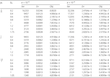
4 Numerical experiments

In this section, we apply the proposed iterative algorithm (3.39) to solve the famous LASSO problem [42]. All the experiments are performed on a standard Lenovo Laptop with Intel (R) Core (TM) i7-4712MQ 2.3 GHZ CPU and 4 GB RAM. We run the program with MATLAB 2014a.

Let us recall the LASSO problem:

min x∈Rn 1

2Ax–b

2 2

s.t.x1≤t,

(4.1)

whereA∈Rm×n,b∈Rm, andt> 0. DeﬁneC:={x|x1≤t}, by using the indicator

func-tion, we see that (4.1) is equivalent to the following unconstrained optimization problem:

min x

1

2Ax–b

2

2+δC(x), (4.2)

which is a special case of the general optimization problem (1.5). Letf(x) = 1₂Ax–b2₂ andg(x) =δC(x), then we can apply iterative algorithm (3.39) to solve (4.2). Notice that

the gradient off(x) is∇f(x) =AT₍_Ax_–_b_{) and the Lipschitz constant of}_∇_f _is_L_:=_A2_.

Besides, the proximity operator of indicator functionδC(x) is the orthogonal projection

onto the closed convex setC. Although it has no closed-form solution, it can be calculated in a polynomial time.

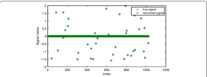
In the tests, the true signalx∈Rnhasknon-zero elements, which is generated from uni-form distribution in the interval [–2, 2]. The system matrixA∈Rm×nis generated from standard Gaussian distribution. The observed signalbis given byb=Ax. In the experi-ment, we setm= 240,n= 1024, andk= 40. The stopping criterion is deﬁned as

xk+1–xk2 xk2 ≤

ε, (4.3)

whereε> 0 is a small constant. We test the performance of the proposed iterative algo-rithm with diﬀerent choices of the step sizeγkand the relaxation parameterλk. For