2018 International Conference on Computer, Communication and Network Technology (CCNT 2018) ISBN: 978-1-60595-561-2
The Design and Implement of Propagation Path-Loss Model over
Sea-Surface under HF
Xiao-jian ZHENG
1, Yu-hui HONG
2,
Lei SHI
3,*and Lei ZHAO
41
School of Microelectronics, Xidian University, Xi’an, China
2
School of Computer Science and Technology, Xidian University, Xi’an, China
3School of Aerospace Science and Technology, Xidian University, Xi’an, China
4
School of Information, Xi’an University of Finance and Economics, Xi’an, China
*Corresponding author
Keywords: Multi-hop Propagation, Transmission Loss, Rough sea surface, PPLM.
Abstract. A new algorithm “Propagation Path-Loss Model” (PPLM) is introduced in this paper. As a correction coefficient and equivalent reflection coefficient are introduced to simulate the reflection loss of calm and rough sea-surface, a mathematical prediction model of sea-surface propagation is devised. This model focus on the analysis of propagation path and transmission loss of skywave, including the propagation loss in free space and ionosphere and reflection loss over the sea-surface. PPLM permits calculating the propagation losses and evaluating propagating capacity of a certain environment by predicting the propagation distance and maximum hops of signal at a certain power. It also can be utilized to predict the communication time based on a geometrical model of skip zone. All the implements indicates that the model is effective and functional.
Introduction
Modeling of propagation path and transmission loss on sea-surface propagation of skywave are of great importance to real applications. Generally, for frequencies below the maximum usable frequency (MUF), sky wave from a ground source reflect off the ionosphere back to the earth and reflect again, traveling in the form of Multi-hop.
However, sea-surfaces are changing all the time. Ocean turbulence will alter the local permittivity and permeability of the ocean and change the height and the angle of the reflection surface, which leads to changes of reflection loss. Several studies and researches have been made on ground wave propagation [1-2], and some focus on the ground wave propagation of terrain like reference[3]. In these papers, the sea roughness effect on skywave propagation is not investigated.
This paper introduces a new model Propagation Path-Loss Model for the HF sky-wave propagation over sea surface based on empirical formulas derived from a series of inspiring measurements. PPLM permits calculating the propagation losses between two generic points using a fast algorithm without enormous computational complexity. It can be utilized to evaluate propagating capacity of a certain environment and predict the propagation distance or maximum hops of signal at a certain power. It can also be employed to predict the communication time. The formulation and derivation are given in Chapter two and three implements of PPLM are given in Chapter 3.
Model Establishment
Propagation Loss
Figure 1. Propagation Path Profile.
Many physical causes will leads the transmission loss during the sky wave propagation. For simplicity, we need only consider four major loss. Transmission Loss can be determined as follows:
(1)
where is the free space loss; is loss caused by ionosphere absorption; is the sea reflection
loss; is for extra system loss.
Assume that the direction of an omnidirectional antenna, some tedious manipulation yields [4]
(2) where f is the frequency in MHz, D is the effective flat-earth range in Km, and n is the number of hops, is the earth's radius (6370km), is the take-off angle.
(3) where is magnetic rotation frequency at a certain height, for example: for the height of 100 km, take 1.4M; is the incident angle.
The is associated with the local time T (hour) of the reflection point and can be estimated from Figure 2:
Figure 2. -T Broken line.
When it comes to the ground reflection loss, the ground reflection loss for multi-hop rays depends
on the reflection coefficient of the rays.
(4) where is the power of incident wave and is the output power; Notice that the Γ is
reflectance and is the reflection coefficient.
Derivation and Correction of
Now we turn to the derivation of . In this paper, we multiply the reflection coefficient of smooth surface by a correction factor to approximate the reflection coefficient of rough surface. Many factors like antenna directivity inhibition roughness, and Earth curvature can be taken into account. In the engineer calculation, it suffices to just introduce the roughness correction factor .
Therefore, the equivalent reflection coefficient denoted as is created, we have
(5) where is the reflection coefficient of smooth surface; is the roughness correction factor and its
Figure 3. Path Profile.
Expression is given by the International Radio Consultative Council (CCIR) as below, where I0 is zero-order modified Bessel function; h is root-mean-square of surface height in first Fresnel zone centered on reflection point[6-7].
(6) Consequently, we have
(7)
where is the reflection loss of a rough surface. Now all the equations we have derived in this section depicts a quantitative and comprehensive process of transmission loss during the propagation.
Implement of PPLM
In actual applications, PPLM can be applied for predictions and screened optimization schemes. For example, if the communication distance is required, the optimal launch elevation Angle can be obtained through the model aiming to a minimal energy consumption with less hops. In this chapter, the simulation environment and parameters for numerical solution are set up to show the detailed description of the three uses of PPLM.
Evaluating Propagating Capacity
Experience tells us that the refraction loss of a calm sea is greater than that of a turbulent sea. Here, the PPLM model verifies this. By using PPLM, the loss of one single hop is calculated respectively on a calm sea and a turbulent sea, respectively. Now that h is root-mean-square of the height of sea surface, it can be given in light of Philips Wave Model [5]
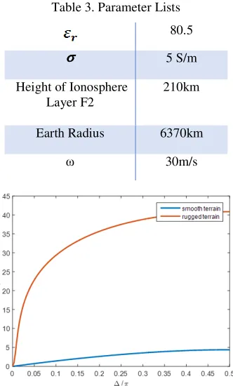
Table 3. Parameter Lists
80.5
σ σ σ
σ 5 S/m
Height of Ionosphere Layer F2
210km
Earth Radius 6370km
ω 30m/s
Figure 4. Comparison of calm sea surface and turbulent sea surface.
While keeping other condition totally the same (at the same time, region, ionosphere, and first three
loss items are remain the same) just changing the take-off angle, four -∆/π curves was obtained, shown in Figure 4.
The propagation ability order is: Calm Sea > Turbulent Sea.
Resolving Maximum Number of Hops
As the noise power at receiver can be computed by noise factors by definition bellow, propagation loss can be calculated by PPLM, the maximum number hops with different take-off angles can be figured out.
(9) where is the noise figure, which can be transformed in dB by ; is available noise power from the equivalent lossless antenna and its expression in dB is ; k is the
Boltzmann constant equaling , is the reference temperature (K) and we take ; b is the noise power bandwidth of the receiving system(Hz). By looking at the table in [6], we can get that . According to the definition of external noise, the noise power of receiving point can be obtained without considering the antenna loss. Thus, we have [7]
Figure 5. Variation of Maximum Hops. Figure 6. Loss in Free Space with ∆/πHop Distance.
Figure 5 gives the maximum number of hops under different take-off angles. Take the point of Δ =45, the signal can take 3 hops before being submerged by noise, its hop distance is 1078km while the loss in free space is 119.1dB.
By increasing the Δ, the maximum number increase exponentially in magnitude. This can be explained by Figure 6. As the Δ arises, the path length of single hop in free space becomes shorter,
which leads the decrease of and consequently signal can take more hops.
Moving Ships Problem
Predicting the communication time of a moving ship is also a very common practical problem. Taking the ground wave into accounts, the cover scale of ground wave is limited with a skip zone appears, which is located between regions that ground wave cannot reach while sky wave has hopped across at the first hop. For HF radio communication, the scale of skip zone is determined by antenna and radiation characteristics (including antenna radiation elevation, gain, equipment power, etc.) The skip zone and track of sky wave are presented in Figure 7.
According to the geometric relations and cosine theorem, we have
; (11) Where A is the radius of the earth, ∆ is the elevation angle; H is the height of reflection point on the
ionosphere. Solving the oblique distance y and the central angle Θ of the reflection, the great-circle
distance x is written as
(12)
Figure 7. Propagation Profile. Figure 8. Sky wave transmission geometry diagram.
In such a case, we have the coverage scale of sky wave S
(13)
Conclusion
PPLM is extremely multifaceted and inclusive while the model keeps concise by efficient simplifications. The numerous calculation point out that the theoretical results obtained from the above propagation models are similar to the actual results. We can draw a conclusion that the roughness of sea surface plays a determined role in skywave propagation. However, by using PPLM, we can analyze factors like roughness and their influence on sky wave propagation directly. Besides, PPLM effectively predicts the skywave propagation over sea-face and shows its multiple functions in sailing communication.
Reference
[1] Shang H Y, An J P, Lu J H. HF ground-wave over rough sea-surface and HF propagation prediction model ICEPAC[C]// Global Mobile Congress. IEEE, 2009:1-4.
[2] C. Bourlier, G. Kubické. HF ground wave propagation over a curved rough sea surface[J]. Waves in Random & Complex Media, 2011, 21(1):23-43.
[3] Rossano R M, Sebastiani M S. Measurements and propagation models of HF ground-wave propagation over irregular terrain and HF sky-wave propagation[C]// Antennas and Propagation, 2001. Eleventh International Conference on. IET, 2002:388-392 vol. 1.
[4] Academy, D. N., & Dalian. (2009). Research on the feasibility of shortwave communication at sea under the condition of atmosphere yawp. Ship Electronic Engineering.
[5] Harbers, G., Mueller, G., Zhou, L., Craford, M. G., Krames, M. R., & Shchekin, O. B., et al. (2007). Status and future of high-power light-emitting diodes for solid-state lighting. Journal of Display Technology, 3(2), 160-175.
[6] Recommendation ITU-R P.372-13. (2016). P Series Radiowave propagation, from https://www.itu.int/dms_pubrec/itu-r/rec/p/R-REC-P.372-13-201609-I!!PDF-E.pdf/
[7] Hu Xibin, & Li Hao. (2010). A Mathematical Model for Calculating Atmospheric Radio Noise. Military Communications Technology (1).