Reduction Rules for Petri Net with Inhibitor Arcs Based Representation for Embedded Systems

2019 International Conference on Computer Science, Communications and Big Data (CSCBD 2019) ISBN: 978-1-60595-626-8

Reduction Rules for Petri Net with Inhibitor Arcs Based Representation

for Embedded Systems

Chuan-liang XIA

, Wei ZHANG and Zhao-cheng WANG

School of Computer Science and Technology, Shandong Jianzhu University, Jinan 250101, China *Corresponding author

Keywords: Petri net, Reduction, Inhibitor arc, Embedded system modeling, Total-equivalent.

Abstract. Petri-net-based Representation for Embedded Systems (PRES+) can describe embedded systems. To improve the modeling ability of PRES+, we add inhibitor arcs to the PRES+ model. Then, Petri net with Inhibitor arcs based Representation for Embedded Systems (PIRES+) is obtained. However, the state space explosion problem is a disadvantage for PIRES+’s ability to model and verify complex embedded systems. In order to solve this problem, reduction rules are proposed. Under certain conditions, these reduction rules preserve total-equivalence.

Introduction

Embedded systems have many applications, such as medical devices, network switches, communication devices and the Internet of Things, in everyday life. High requirements on reliability, correctness, and real-time behavior, are characteristics of embedded systems [1]. It is important to focus on how to model and guarantee correctness of embedded systems.

In the literature, there exist several models to describe embedded systems, such as finite state machines, data flow graphs, and Petri nets. The Petri-net-based Representation for Embedded Systems (PRES+) is an excellent methodology for modeling, verification, and analysis of embedded systems [2-6].

In order to design embedded systems, Cortés et al. [2] presented a formal computational model for embedded systems based on PRES+. Karlsson et al. [3] proposed a method for PRES+ to integrate with component based system level design. Xia et al. [5, 6] proposed a refinement method and a synthesis method for PRES+ model to preserve several dynamic properties.

The addition of inhibitor arcs can enhance Petri net’s modeling ability [7, 8]. In order to improve the modeling and verifying ability of PRES+, we add inhibitor arcs to the PRES+ model. Then, Petri net with Inhibitor arcs based Representation for Embedded Systems (PIRES+) is obtained. However, the state space explosion is a tedious problem for PIRES+ to model and verify complex embedded systems.

To resolve state space explosion problem of Petri nets, many researchers have used transformation approaches. There exist three popular transformations in the literature, namely reduction, synthesis, and refinement.

Petri net based reduction is an effective approach to system design and verification. As for reduction method, H. Boucheneb et al. [9] proposed a partial order reduction technique for time Petri

nets (TPN). Berthomieu et al. [10] presented an approach to reduce the number of places and

transitions. For system specified in PRES+, Xia [4] presented a set of reduction rules. Under certain conditions, the reduced PRES+ model preserves reachability, timing and functionality.

The major motivation of this paper is to solve PIRES+’s state space explosion problem and to model embedded systems. We will propose the concept of PIRES+, and present two kinds of reduction rules for PIRES+. Under some constraints, these rules preserve total-equivalence. These results are useful for investigating the properties of PIRES+ reduction nets and establishing models for complex embedded systems.

model. Section 3 presents the reduction rules and investigates the preservation of total-equivalence. Section 4 illustrates the efficiency of these reduction rules with an applicable example. Conclusions are drawn in Section 5.

Preliminaries

In this section, first, we will review the key notions of PRES+. Some more general analysis of the PRES+ model can be found in [2]. Second, we will propose the concept of PIRES+ and the corresponding notion of total-equivalence for PIRES+.

A PRES+ model is a five-tuple N = (P, T, FI, FO, M0), where P is a finite set of places; T is a finite set

of transitions; FI  P  T is a finite set of input arcs;Fo  T  P is a finite set of output arcs;M0is the

initial marking. The token carries time and data information. For every transition, there exists a transition function, a minimum transition delay and a maximum transition delay.

If inhibitor arcs are added to the PIRES+ model, then Petri net with Inhibitor arcs based Representation for Embedded Systems (PIRES+) is obtained.

Definition 2.1 A PIRES+ model is N = {P, T, FI, FO, I, M0}, where P ={p1 ,p2 ,…,pm} is a finite set

of places; T ={t1 ,t2 ,…,tm}is a finite set of transitions; FI  P  T is a finite set of input arcs; FO  T 

P is a finite set of output arcs; I  P  T(I  F=)is a finite set of inhibitor arcs; M0 is the initial

marking. A token is a park k=<v, r>, where v is token value, r is the token time.

A transitioncan only fire if all its inhibitor places are empty. Graphically, an inhibitor arc connects

a place to a transition, and the arc ends with an empty circle on the transition side. The rest constraints are the same as those of PRES+ model.

The validity of a reduction depends on the concept of equivalence. Two equivalent systems are not necessarily the same but have properties that are common on both of them. In order to investigate property preservation of the reduction rules, we propose the concept of total-equivalence for PIRES+.

Definition 2.2 Two PIRES+ nets N1 and N2 are said to be total-equivalent if and only if: (1) There

exists bijections fin: inP1inP2 and fout: outP1 outP2 that define correspondences between

in(out)-port of N1 and N2;

(2) The intial markings M1,0 and M2,0 satisfy pP1, M1,0(p)=M2,0(fin(p)); qoutP1,

M1,0(q)=M2,0(fout(q));

(3) M1R(N1) satisfy pP1, m1(p)=0, sP1\inP1\outP1, m1(s)=m1,0(s). M2R(N2) satisfy

pP2, m2(s)=m2,0(s), sP2\inP2\outP2, m2(s)=m2,0(s), qoutP1, m2(fout(q))=m1(q), vice versa;

(4) <v1,r1>M1(q), qoutP1, <v2,r2>M2(fout(q)), satisfy v1=v2, r1=r2, vice versa;

(5) The control of firing sequence’s inhibitor arcs of N1 is the same as that of N2.

Reduction Rules

In this section, two reduction rules of PIRES+ are proposed. These rules will preserve total-equivalence.

The Reduction Rule Based on Sequential Places

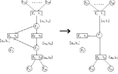
In this section, we investigate the reduction rule of PIRES+ based on sequential places (RP).This

reduction rule allows for merging several sequential places with only one transition between every

neighboring place into one place. For example in Figure 1, there exists only one transition t2 between

place p1 and p2, i.e., p1 is the unique input place of t2, and p2 is the unique output place of t2. p1 and p2

do not share input transitions. p1 and p2 inhibit the same transition tu.

Definition 3.1 (Reduction based on sequential place: RP) Suppose N1={P1,T1,FI1,FO1,I1,M1,0} and

N2={P2,T2,FI2,FO2,I2,M2,0} are two PIRES+ models. (N1,N2)RP if there exists input places Pi  P1

P2, where Pi={pi1, pi2, …, pim}, output places Po  P1 P2, where Po={po1, po2, …, pon}, p1, p2P1\(Pi

Po), p’ P2\P1, t2T1, ( p1,tu)I1, ( p2,tu)I1, such that:

(6) I1.(t)=  ( where transition t has not inhibitor arcs);(7) M1,0 (where M1,0 isthe initial marking of

N1), piPi, M1,0(pi); poPo, M1,0(po)=; (8) There are transition functions f1 and f2 associated to

t1 and t2 respectively; (9)There are transition delays [a1,b1] and [a2,b2] associated to t1 and t2

respectively.

N2: (10) P2 = (P1\{p1,p2}){p’}; (11) T2 =T1\ {t2}; (12) FI2 = (FI1(P2T2))({ p’} p2.); (13) FO2 =

(FO1(T2P2))(((.p1.p2)\{t2}){p’}); (14) xT2, if {p1,p2}I1(x), then

I2(x)=I1(x)\{p1,p2}{p’}, and if {p1,p2}I1(x)=, then I2(x)=I1(x); (15) M2,0 = M1,0 (where M2,0 is the

initial marking of N2); (16) The transition function of t1 is f, where f=f2 f1; (17) The transition delay of

t1is [a, b], where a=a1+a2,b=b1+b2; (18) The rest constraints of N2 are the same as those of N1.

Figure 1. An example of reduction rule RP.

Theorem 3.1 SupposeN1 and N2 are two PIRES+ nets which satisfy (N1, N2)RP. Then N1 and N2

are total-equivalent.

Proof Since (N1, N2)RP, by Definition 3.1, there exist bijections fin: inP1 inP2, fout: outP1

outP2, inP1= inP2=Pi, outP1 = outP2 = Po. Obviously, fin (fout) defines correspondences between

in(out)-port of N1 and N2. The initial marking M1,0 and M2,0 satisfy piPi, M2,0(pi)= M1,0(pi),

poPo, M2,0(po)= M1,0(po)=. M1R(N1), piPi, m1(pi)=0; pP1\(PiPo), m1(p)=m1,0(p).

Since there exists transition function f1 and f2 associated to t1 and t2 in N1, by Definition 3.1, there

exists transition function f associated to t1 in N2, and f=f2f1. There are delays [a1, b1] and [a2, b2]

associated to t1 and t2, by Definition 3.1, there is transition delay [a, b] (where a=a1+a2, b=b1+b2)

associated to t1 of N2. Then M2R(N2), piPi, m2(pi)=0; pP2\(PiPo), m2(p)=m2,0(p), poPo,

m2(fout(po))= m2(po) and vice versa. From above, poPo, <v1,r1>M1(po), there exists <v2,r2>

M2(po) such that v1= v2, r1= r2 and vice versa.

The firing of inhibited transitions in two nets depends on the post-set places of t1 and the pre-set

places of t3. It is easy to see that inhibited transitions are firing in the same situation in N1 and N2.

Thus, N1 and N2 are total-equivalent.

Reduction Based on Sequential Transitions

In this section, we investigate the reduction rule of PIRES+ based on sequential transitions (RT). This

reduction rule allows for merging several sequential transitions with only one place between every

neighboring transition into one transition. For example in Figure 2, there exists only one place p1

between transition t1 and t2, i.e., t1 is the unique input transition of p1, and t2 is the unique output

transition of p1. Both t1 and t2 are inhibited by place p2.

Definition 3.2 (Reduction based on sequential transitions: RT) Two PIRES+ net are

N1={P1,T1,FI1,FO1,I1,M1,0}, N2={P2,T2,FI2,FO2,I2,M2,0}. (N1,N2)RT if there exists input places

PiP1P2, where Pi={pi1,pi2,…,pim}, output places PoP1P2, where Po={po1,po2,…,pon},

p1,p2P1\(PiPo), p1P1\P2, transition t1,t2T1, t’T2, (p2, t1)I1, (p2,t2)I1, (p2, t’)I2 such that:

N1: (1)p1P1\P2,p2P1\P2; (2) t1T1\T2,t2T1\T2; (3) . p1= {t1}; (4) p1. ={t2},. t2={ p1}; (5) t1.

M1,0(pi); poPo, M1,0(po)=; (9)f1 and f2 are transition functions of t1 and t2 respectively;

(10)[a1,b1] and [a2,b2] are transition delays of t1 and t2 respectively.

N2: (11)t’T2; (12) T2=T1{t1,t2}+{t’}; (13) FI2=(FI1(P2T2))(.t1{t’}); (14)

FO2=(FO1(T2P2))({t’}((t1.t2.)\{p1})); (15)xT2, if xt’, then I2(x)=I1(x)\{p1}, and if x=t’, then

I2(x)=I1(t1)\{p1}; (16)xP2, if xt2., then M2(x)=M1(x)\ M1(p1), and if x t2., then M2(x)=M1(x); (17)

The transition function of t1 is f, where f=f2 f1; (18) The transition delay of t1 is [a, b], where a=a1+a2,

and b=b1+b2; (19) M2,0= M1,0 (where M2,0 is the initial marking of N2); (20) The rest constraints of N2

are the same as those of N1.

Figure 2. An example of reduction rule RT.

Theorem 3.2 N1 and N2 are two PIRES+ nets which satisfy (N1, N2)RT, then N1 and N2 are

total-equivalent.

Proof Since (N1, N2)RT, by Definition 3.2, there are bijections fin: inP1 inP2, fout: outP1 outP2,

inP1= inP2=Pi, outP1=outP2=Po. Obviously, fin(fout) defines correspondences between in(out)-port of

N1 and N2. The initial marking M1,0 and M2,0 satisfy piPi, M2,0(pi)= M1,0(pi), poPo, M2,0(po)=

M1,0(po)=.

M1R(N1), piPi such that m1(pi)=0; pP1\(PiPo), m1(p)=m1,0(p). Since f1 and f2 are

transition functions of t1 and t2 in N1, by Definition 3.2, there is transition function f associated to t1 in

N2, and f=f2f1. Since [a1, b1] and [a2, b2] are transition delays of t1 and t2, respectively in N1, by

Definition 3.2, there is transition delay [a, b] associated to t1 in N2, where a=a1+a2, and b=b1+b2. Then

M2R(N2), such that piPi, m2(pi)=0; pP2\(PiPo), m2(p)=m2,0(p),poPo, m2(fout(po)) =

m2(po) and vice versa. From above, <v1,r1>M1(po), there exists <v2,r2> M2(po) such that v1= v2,

r1= r2 and vice versa. The firing of inhibited transitions in two nets both depends on p2. It is easy to see

that inhibited transitions are firing at the same situation in N1 and N2. Then, by Definition 2.2, N1 and

N2 are total-equivalent.

Applications

In this section, two reduction rules of PIRES+ are proposed. These rules will preserve total-equivalence.

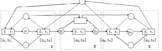
Figure 3. An embedded processing system model.

be proposed in this section. An embedded processing system model will be reduced by using above reduction rules for PIERS+ model. This embedded system model (Figure 3) includes three parts. Part 1 represents embedded processing subsystem 1. Part 2 describes the buffer, and part 3 represents embedded processing subsystem 2. In order to improve the verification efficiency, the model will be reduced by applying the above reduction rules.

The reduced PIRES+ model (Figure 4) is obtained by using the reduction rule RT. In Part 1,

transition t1 and t2 are merged as t6. In Part 3, transition t4 and t5 are merged as t7. The transition

function of t6 isf6, wheref6=f2 f1. The transition function of t7 isf7, wheref7=f4 f5. The transition delay

of t6 is [a6, b6], where a6=a1+a2 and b6=b1+b2. The transition delay of t7 is [a7,b7], where a7=a4+a5 and

b7=b4+b5.Inhibitor arcs inhibit transition t6 and t7, respectively.

Figure 4. The reduced model.

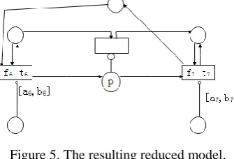
The resulting reduced model (Figure 5) is obtained by using the reduction rule RP. Place p2 and p3

are merged as place p. The transition which is inhibited by p2 and p3 is inhibited by p.

Figure 5. The resulting reduced model.

The original model is reduced by reduction rules R2 and R1. By Theorem 3.2 and Theorem 3.1, the

resulting reduced model and the original model are total-equivalent.

Conclusions

In order to enhance the PRES+’s ability to model and verify complex embedded systems, we extend PRES+ to PIRES+ by adding inhibitor arcs. But the state space explosion problem is somewhat tedious for PIRES+ to specify and analyze large complex embedded systems. To solve this problem, we present two kinds of reduction rules for PIRES+. These reduction rules preserve total-equivalence, and can be nicely used to solve design problem in embedded systems. Other more general reduction approaches for PIRES+ should be investigated in the future.

Acknowledgement

References

[1] M. Ashjaei, N. Khalilzad, S. Mubeen, Modeling, designing and analyzing resource reservations in distributed embedded systems, M. Alam et al. (eds.), Real-Time Modeling and Processing for Communication Systems, Lecture Notes in Networks and Systems 29 (2018) 203-256.

[2] L. A. Cortés, P. Eles, Z. Peng, Modeling and formal verification of embedded systems based on a Petri net based representation, J. Syst. Arch. 49 (2003) 571-598.

[3] D. Karlsson, P. Eles, Z. Peng, Formal verification of component-based designs, Des. Autom. Embed. Syst. 11 (2007) 49–90.

[4] C. Xia, Reduction rules for Petri net based representation for embedded systems, J. Front. Compu. Sci. & Tech. 2 (2008) 614-626.

[5] C. Xia, Property preservation of refinement for Petri net based representation for embedded systems, Cluster Compu. 19 (2016) 1373-1384.

[6] C. Xia, B. Shen, H. Zhang, Y. Wang, Liveness and boundedness preservations of sharing synthesis of Petri net based representation for embedded systems, Comput. Syst. Sci. & Eng. 33 (2018) 345-350.

[7] S. Ivanov, E. Pelz, S. Verlan, Small universal non-deterministic Petri nets with inhibitor arcs, H. Jürgensen et al. (Eds): DCFS 2014, LNCS 8614 (2014) 186-197.

[8] M. Alqarni, R. Janicki, On interval process semantics of Petri nets with inhibitor arcs, R. Devillers and A. Valmari (Eds.): PETRI NETS 2015, LNCS 9115 (2015) 77-87.

[9] H. Boucheneb, K. Barkaoui, K. Weslati, Delay-dependent partial order reduction technique for time Petri nets, A. Legay and M. Bozga (Eds.): FORMATS 2014, LNCS 8711 (2014) 53-68.