Towards Excited Radiative Transitions in Charmonium

(1)

Doctoral Thesis

Towards Excited Radiative

Transitions in Charmonium

Author:

Cian O’Hara

Supervisor:

Prof. Sin´ead Ryan

A thesis submitted in fulfilment of the requirements

for the degree of Doctor of Philosophy

in the

School of Mathematics

(2)

Declaration of Authorship

I declare that this thesis has not been submitted as an excercise for a degree at this or any other university and is entirely my own work.

I agree to deposit this thesis in the University’s open acess institutional repository or allow the Library to do so on my behalf, subject to Irish Copyright Legislation and Trinity College Library conditions of use and acknowledgement.

Signed:

Date:

(3)

Abstract

Towards Excited Radiative Transitions in Charmonium

by Cian O’Hara

In this thesis lattice QCD is utilised to investigate the spectrum of charmonium and charmed mesons with the aim of working towards investigating radiative tran-sitions between excited states in the charmonium spectrum. Results are presented from a dynamical Nf = 2 + 1 lattice QCD study of the excited spectrum of Ds

and D mesons at a single lattice spacing with pion mass Mπ = 236 MeV, which

has been published in reference [1]. A robust determination of the highly excited spectrum of states, up to spin J = 4, was achieved with the use of distillation and the variational method. A comparison with earlier studies of the spectra on lattices with heavier light quarks was performed and the spectrum was found to have little dependence on the light quark mass. Results from an investigation into radiative transitions in the charmonium spectrum are also presented. A number of transitions are investigated and compared to experiment where possible. Three point correlation functions with a vector current insertion are calculated for a range of source and sink momenta allowing for the extraction of radiative form-factors for a wide range of Q2 _{values. In particular, the transition}_J/ψ _→_η

cγ was

(4)

Acknowledgements

Firstly, I would like to thank Prof. Sin´ead Ryan for all of the advice and supervi-sion over the years during the course of this project, as well as her many helpful comments on this thesis, without which it would have never been completed. I would also like to especially thank Christopher Thomas, David Wilson and Gra-ham Moir, who all gave up so much of their time over the past four years whenever help was needed.

I would like to thank Mike Peardon and the rest of the Hadron Spectrum Collab-oration, for providing the resources and computational infrastructure which was necessary for this work to be completed.

My officemates David Tims and Argia Rubeo, are owed many thanks for making these four years all that more enjoyable and for all the interesting discussions, academic or otherwise.

I would like to thank my girlfriend Manya and my mother Linda whose support helped me get to where I am today.

Finally I would like to thank the school of maths and the Irish Research Council for providing the funding which allowed this work to be performed.

(5)

List of Figures

2.1 The link variablesUµ(n) and U†

µ(n) . . . 14

2.2 An elementary plaquette, Uµν(n) . . . 15

2.3 The dimension six 2×1 rectangular operator . . . 20

2.4 The clover operator, Gbµν(n) . . . 22

3.1 A schematic representation of a correlation function . . . 36

3.2 Principal correlators in the T₁− irrep of the Ds spectrum . . . 40

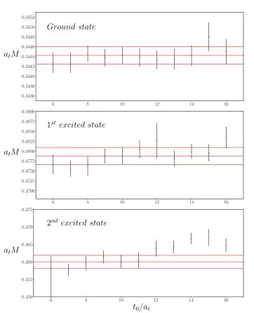
3.3 t0 dependence of the energy in the T1− irrep of the Ds spectrum . . 42

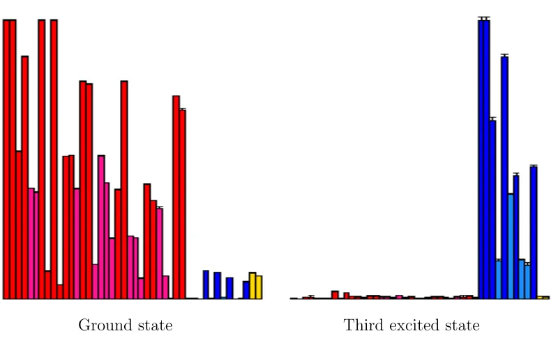
3.4 Operator overlaps for states in the T1− irrep of the Ds spectrum . . 44

3.5 Comparison of operator overlaps for states across the A−2, T − 2 and T1− irreps in the Ds spectrum . . . 45

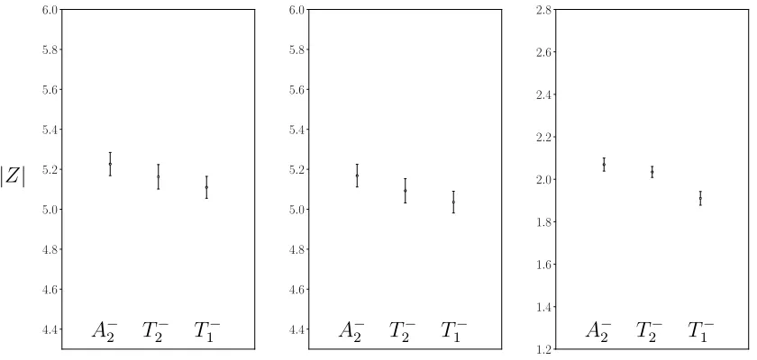
3.6 Comparison of absolute values for the operator overlaps, |Z|, across irreps A−₂, T₂− and T₁− for the Ds meson. . . 45

4.1 Dispersion relation for the ηc and D meson measured on themπ ∼ 240 MeV lattice . . . 49

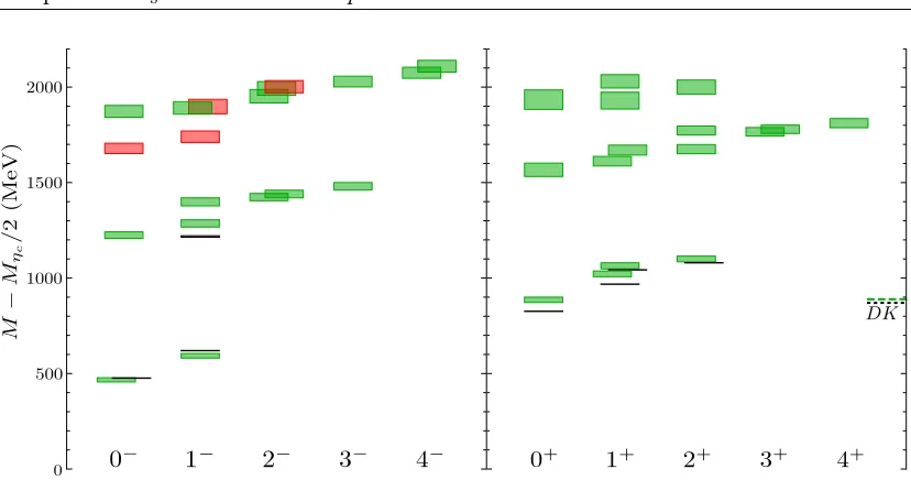
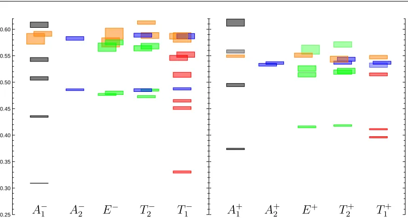
4.2 Ds meson spectrum in lattice units labelled by lattice irrep, ΛP . . 51

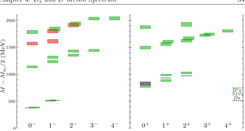
4.3 Ds meson spectrum labelled byJP . . . 52

4.4 D meson spectrum in lattice units labelled by lattice irrep, ΛP _{. . . 53}

4.5 D meson spectrum labelled byJP _{. . . 54}

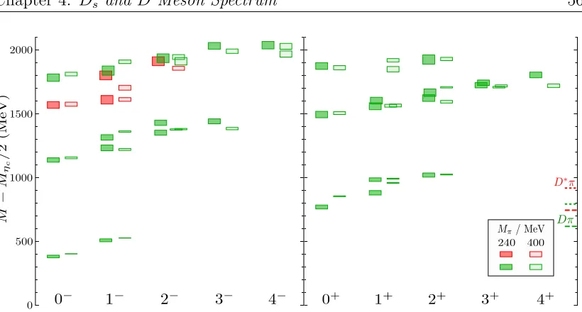
4.6 Comparison of the Ds meson spectrum for two different light quark masses labelled by JP _{. . . 55}

4.7 Comparison of the D meson spectrum for two different light quark masses labelled by JP _{. . . 56}

5.1 A schematic representation of a three point correlation function . . 65

5.2 Principal correlator comparison using improved and unimproved operators for theηc . . . 71

5.3 Principal correlator comparison using improved operators for an excited state. . . 72

5.4 Temporal ηc form-factor for ∆t= 40 and ∆t= 32 . . . 73

5.5 A selection of correlation functions plotted for a range of different source and sink momenta . . . 74

5.6 The temporalηc form-factor F(Q2) vsQ2 . . . 75

5.7 Zero momentum transfer ηc form-factor . . . 76

(8)

List of Figures viii

5.8 Comparison of the ηc spatial and temporal form-factors, using the improved and unimproved currents . . . 79 6.1 Charmonium spectrum calculated on themπ ∼391 MeV lattice . . 82 6.2 Dispersion relation for the ηc meson measured on the mπ ∼ 391

MeV lattice . . . 84 6.3 ηc form-factor for unimproved temporal and spatial currents . . . . 86 6.4 ηc form-factor for improved temporal and spatial currents . . . 88 6.5 χc0 form-factor for improved temporal and spatial currents . . . 90 6.6 η0

c form-factor for improved temporal and spatial currents . . . 92 6.7 Form-factor F(Q2_{) vs} _Q2 _{for the} _J/ψ _→ _η

c transition using the improved spatial current . . . 95 6.8 Comparison of lattice values for the decay width Γ(J/ψ_→ηcγ) . . 96 6.9 Form-factor E(Q2_{) vs} _Q2 _{for the} _χ

c0 → J/ψ transition using the improved spatial current . . . 98 6.10 Principal correlators for ηc,η0

(9)

List of Tables

1.1 Possible JP C _and _JP _{values allowed from simple quark models} _{. . .} ₅ 2.1 Action parameters. . . 24 3.1 Gamma matrix quantum numbers and naming scheme . . . 30 3.2 Subduction pattern for various spins into the irreducible

represen-tations of the octohedral group . . . 33 3.3 Subduction coefficients for (J = 1)_→T1 . . . 33 4.1 Details of the lattice gauge field ensembles used in the Ds and D

meson spectrum study . . . 48 4.2 Mixing angles for the lightest pairs of 1+_{, 2}− _{and hybrid 1}− _states

in the charm-strange and charm-light sectors on two ensembles . . . 57 5.1 Allowed lattice momenta on a cubic lattice in a finite cubic box,

along with the corresponding little groups for relevant momenta . . 67 5.2 Rotations, Rref, for rotation ˆRφ,θ,ψ = e−iφ

ˆ

Jz_e−iθJˆy_e−iψJˆz _{that takes}

(0,0,_|~p_|) to ~pref . . . 68 5.3 Subduction coefficients, S_Λη,λ˜_,µ, for _|λ_{| ≤}4 . . . 69 6.1 Details of the lattice gauge field ensembles used in the study of

radiative transitions in charmonium . . . 83 6.2 Summary of the masses for theηc, J/ψ andχc0 found on the lattice,

as well as their experimental values . . . 94 B.1 Summary of the energies of the Ds meson spectrum presented in

Figure 4.3 . . . 110 B.2 Summary of the energies of the D meson spectrum presented in

Figure 4.5 . . . 110 B.3 ηc form-factor values . . . 111 B.4 χc0 form-factor values . . . 112 B.5 η0

c form-factor values . . . 113 B.6 J/ψ→ηc and χc0 →J/ψ transition form-factor values . . . 114

(10)

(11)

Chapter 1 Introduction

From as far back as the ancient Greeks, mankind has sought to understand the building blocks of the material world in which we live. The idea that all matter is made up of indivisible units dates back to the 5th century BC. Since then our understanding of the nature of these atoms, from the Greek, atomon, meaning indivisible, has gone through many paradigm shifts. Due to the work of many experimental physicists, primarily Ernest Rutherford, John Cockcroft and Ernest Walton, in the early 20th century, the modern idea of the atom comprised of other more fundamental constituents, the electron, the proton and the neutron, emerged. These physicists pioneered the idea of accelerating particles to very high energies and smashing them together to see what they are made of.

Our current understanding of the fundamental constituents of matter dates to the 1960s when Murray Gell-Mann and George Zweig proposed independently the idea of the quark. Motivated by the ideas of SU(3) flavour symmetry, or the Eightfold Way, six quarks were envisioned and subsequently discovered over the course of 30 years, with the top quark being the last to be experimentally confirmed in 1995 [2, 3]). To this day, particle physicists around the world are building accelerator experiments reaching higher and higher energies than ever before in an attempt to further probe these fundamental matter particles.

The idea of a force between these building blocks dates to Issac Newton in the sixteenth century. In the ”Philosophiae Naturalis Principia Mathematica” [4], he introduced the gravitational force which acts between any pair of massive objects.

(12)

Chapter 1. Introduction 2

In the 19th century James Clerk Maxwell united the ideas of elctricity and mag-netism into the electromagnetic force. Then in the 20th century Albert Einstein revolutionised our understanding of gravity yet again with his theory of general relativity [5]. We now know of two other fundamental forces that govern the way subatomic particles interact. The strong nuclear force, which binds quarks to-gether in nucleons and the weak nuclear force which is responsible for radioactive beta decay. In 1968 Sheldon Glashow, Abdus Salam and Steven Weinberg unified this weak force with the electromagnetic force into the electro-weak force [6–8]. The Standard Model of particle physics is the name given to the current theory describing the known elementary particles and the three aformentioned funda-mental forces, the strong, weak and electromagnetic forces. Gravity, described by Einstein’s general relativity, is as of yet, not included. It is proposed that all four forces may unite into a single force at extremely high energies but such a theory of everything is currently unknown. This would require a quantum theory of gravity, which is well beyond the scope of this thesis.

(13)

The fact that these gluons interact among themselves, leads to what is known as colour confinement. This is the statement that no lone quarks or composite hadronic particles with non-zero colour charge are observed in experiment; ie. the quarks are bound inside composite particles. The simplest colour singlet arrange-ments of quarks consistent with this notion can be grouped into two classes, known asbaryons andmesons, or collectively ashadrons. Baryons consist of three quarks (qqq) while mesons are made of a quark and an anti-quark (qq¯). It also allows for more exotic states such as tetraquarks (qqq¯q¯) or pentaquarks (qqqq¯q¯), in which there is much interest [9]. These states of matter may potentially explain some currently unexplained resonances seen in experiment. However, for the purposes of this thesis we are primarily concerned with mesons containing a charm (c) quark. The relative strength of the theories of QCD and QED can be encapsulated by their gauge couplings. In the case of QED, the fine structure constant,α, describes how strongly charged matter interacts with photons. At energy scales of the order of a hadron mass this takes a value of approximately 1/137. Due to this relatively small coupling, the theory of QED can be accurately described via a perturbative expansion to all orders. Perturbative calculations have had enormous success in calculating QED phenomena, such as the anomolous magnetic moment of the electron, to extremely high precision [10].

On the other hand, the coupling involved in the strong interaction, αS, “runs”

inversely to the energy scale. This asymptotic freedom means that at high energies, the strong force becomes weaker and quarks become essentially free. However at the energy scale of hadrons, αS is of the order one. This strong coupling is where

the strong force derives its name. The fact that this is of the order one means that hadronic interactions via the strong force cannot be accurately described using perturbation theory. Because of this another method to investigate the hadronic bound states of QCD is needed.

(14)

The work presented in this thesis utiliseslattice regularisation, introduced by Wil-son [11]. The use of a lattice as a regulator to investigate the strong force is the basis of the discipline of Lattice QCD. By discretising the theory of QCD on a spacetime lattice the path integral can be estimated explicitly using computa-tional methods, avoiding the need to use perturbation theory. This will allow us to investigate the theory of the strong interaction at the hadronic scale where the cou-pling is large and elucidate the spectrum of hadrons allowed by the theory. Lattice QCD calculations are systematically improvable calculations from first principles allowing for accurate comparison to experiment with well defined sources of error.

1.1 Charm Physics

Any theory of sub-atomic particles is only valid provided it can hold up when com-pared to the empirically observed spectrum of states seen in experiment. With decades of data from accelerator experiments measured, by the 1970s a large “zoo” of experimentally observed particles were known. However it took until the in-troduction of the idea of quarks that any pattern amongst this zoo was obvious. Simple models, describing the various observed particles as strongly bound com-binations of valence quarks had great success in explaining the observed spectrum of states. The discovery of the J/ψ meson, and hence the charm (c) quark, si-multaneously by two different groups in 1974 was the final experimental evidence needed to allow the quark model of hadrons to become widely accepted, [12, 13]. The charm quark is of particular interest as it is substantially heavier than the lighter up, down and strange quarks, allowing it to be described by simple non-relativistic potential models but also light enough that it lives long enough to form observable bound states. In this way it is in a rather unique position and its spectrum can be used to compare experiment to theory.

Since 1974, there have been as many as eighteen experimentally confirmed states in the charmonium spectrum. Charmonium is a meson containing a cquark and its anti particle (¯c), with the aforementioned J/ψ being the first observed meson in the spectrum. There have also been many observed states in the spectrum of charmed-strange mesons (cs¯) known as theDs meson and the charmed-light (c¯l)

(15)

L S J JP C

0 0 0 0−+

1 1 1−−

1 0 1 1+−

1 2,1,0 2++_,₁++_,₀++

2 0 2 2−+

1 3,2,1 3−−_,₂−−_,₁−−

3 0 3 3+−

1 4,3,2 4++_,₃++_,₂++

L S J JP

0 0 0 0−

1 1 1−

1 0 1 1+

1 2,1,0 2+_,₁+_,₀+

2 0 2 2−

1 3,2,1 3−_,₂−_,₁−

3 0 3 3+

1 4,3,2 4+_,₃+_,₂+ Table 1.1: Possible JP C and JP values allowed from simple quark models.

For a long time, a simple model of valence quarks bound together in hadrons was enough to explain the observed spectra. Simply, a meson is a hadronic bound state composed of a quark and anti-quark pair. As quarks are spin 1

2 fermions, the allowed spin S for a meson in its ground state is either 0, when the quarks spins are anti-parallel or 1 when the spins are aligned.

When the the spins are aligned the meson is said to be in a spin triplet state as there are three Sz projections 1,0,-1. If the spins are opposite then there is only

one Sz projection, namely Sz = 0 and the meson is said to be in a spin singlet

state.

Along with this spin angular momentum, the meson can have an orbital angular momentum L. The total spin, J, of the meson is then given as

J =L+S with |L−S| ≤J ≤ |L+S|. (1.1.1)

In this way the mesons can be classified using the familiar spectroscopic notation of the Hydrogen atom, n2S+1_L

J. Along with spin, each meson is also labelled

according to how it transforms under the operations of charge conjugation C and parity transformationsP. The charge and parity quantum numbers are related to the spin of a meson via the following simple formulae.

P = (₋1)L+1_, _C_{= (}

−1)L+S_. _(1.1.2)

(16)

and anti-quark of different flavour, such as the Ds and Dmesons,C is not a good

quantum number and so the states can be labelled by just their JP _numbers.

Using these formulae the allowed states in the spectrum of a meson can naively be predicted as shown in Table 1.1. It is noteworthy that in this model some

JP C _{combinations, such as 0}+−

and 1−+ _{do not appear. These exotic quantum} numbers give rise to what are termedexotic states, and the search for such states is ongoing.

Over the past decade many states that do not fit nicely into these naive classifi-cations have been observed in experiment [14]. Specifically in the case of charmo-nium, the observation of so-calledX, Y, Z states highlight the need for a more com-plete theoretical understanding of the hadronic spectrum, be they hybrid mesons, tetra-quarks or some other hitherto unknown form of matter, [15, 16]. Similarly, in the charm-light sector, states such as theDs0(2317)±andDs1(2460)±have been found to have much narrower widths than expected [17].

In order for QCD to be an accurate description of nature, it must account for these unexplained states seen in experiment. One way to test this is to perform a first principles lattice QCD calculation of the theory and attempt to reproduce the spectrum observed in experiment.

1.2 Lattice Basics

According to Feynman, a field theory with field Φ and relativistic action S[Φ] can be quantised by writing down a path integral. From this one can calculate expec-tation values of the theory’s observables O(Φ) from n-point correlation functions as

h0_|O1(Φ),O2(Φ)...On(Φ)|0i=

1

Z

DΦe−iS[Φ]

O1(Φ),O2(Φ)...On(Φ). (1.2.1)

Z is known as the partition function and is given by

Z = Z

(17)

These expressions involve integrals over all possible field configurations Φ weighted by the Boltzmann factor e−iS[Φ]_{. To make such calculations possible and} mathe-matically well defined one must introduce a regulator, to avoid infrared and ultra-violet divergences. There are many possibilities such as dimensional regularisation or Pauli-Villars regularisation, however this work is performed using lattice regu-larisation [11].

To do this, spacetime is modelled no longer as a continuum but a four dimensional finite sized discrete box of length L, made of points with a finite spacing, a, between them. Matter fields can now only live on the lattice points and the gauge fields live on the links between them. In this way a natural ultraviolet cutoff, 1/a, has been introduced which regulates any momentum integrals. The finite extent of the lattice also acts as an infrared cutoff. Spacetime integrals over the field configurations now become sums over a finite set of lattice field configurations. This allows Eqn. 1.2.1 to be recast as a lattice path integral which is a sum over operators acting on this finite set of lattice field configurations. As it appears in Eqn. 1.2.1, the exponential weighting factor is highly oscillatory. However a Wick rotation may be performed on the Minkowski time coordinate, such thatt _{→ −}iτ. This allows Eqn. 1.2.2 to be rewritten as a Euclidean path integral, where SE is

now the discretised Euclidean action.

Z = Z

DΦe−SE[Φ]_. _(1.2.3)

The lattice regularisation naturally lends itself to computational methods. Monte Carlo importance sampling techniques can be used in the evaluation of any observ-ables computationally. One can generate a large ensemble of lattice configurations in a Markov chain weighted by e−SE which minimise the action and hence

(18)

explored using non-perturbative methods. It also allows the use of many methods from the study of statistical mechanics which can be used to help understand QCD.

1.3 Sources of Error

Introducing a lattice as a regulator and using Monte Carlo estimation techniques to evaluate path integrals will necessarily result in the introduction of statistical and various systematic errors in any lattice calculation. Any result must then have these sources of error under control so as to be able to make contact with experimental results. These various errors can classified as follows:

• Statistical errors - Approximating the path integral shown in Eqn. 1.2.1as a sum to be estimated via Monte Carlo integration introduces statistical errors. These can be reduced by increasing the number of field configurations, N, used and fall off as _√1

N. Errors quoted in this work will be purely statistical.

For more information see Appendix A.

• Discretisation errors - These arise due to discretising the action of the theory on the lattice with finite spacing a. These errors appear in powers of a and can be formally reduced via a procedure known as improvement which will be discussed in Chapter 2. Calculations at smaller a will also reduce these errors but increase the time needed to simulate on a computer.

• Finite volume errors - These arise due to the finite extent L of the lattice. However these errors are proportional to e−M L_{, where} _M _{is the lattice pion}

mass, and so can be mitigated by takingLto be large compared to the mass scale of the system under investigation. Simulating at more than one value of L allows these errors to be quantified.

(19)

• Chiral extrapolation - Due to computational constraints, lattice simulations are often performed using un-physically heavy light quark masses. Simu-lating at multiple quark masses allows for an extrapolation to the physical point, which introduces its own model dependent error. However more re-cently calculations at physical quark masses have started to be performed [18, 19].

• Heavy Quarks - The charm quark was traditionally difficult to simulate on the lattice due to its large massmc compared to the lighter quarks. While it

is light enough to be treated relativistically, finite volume and discretisation effects can become large. Anisotropic lattices allow for a solution where only the temporal spacing is reduced such that mcat 1, without greatly

increasing the computational cost of simulating at small a, however errors involving as will still exist.

Lattice calculations of hadronic spectra are now the definitive way of investigating the theory of QCD in the non-perturbative regime. The accurate description of the energies of low lying states in the QCD spectrum has been an important benchmark of lattice studies for many years. For a recent review see [20, 21]. Recently newer technologies and increased computational power have allowed for studies of higher-lying states and resonances. These studies allow for much more precise determinations than ever before, as well as providing valuable insight into previously unstudied regions such as hybrid or exotic states, [22–25].

In this thesis some topical questions in the charmonium spectrum will be inves-tigated utilising the most up to date technologies and lattices available. Starting with a discussion of QCD in Chapter 2, the technology needed to perform a spec-troscopic calculation on the lattice will be introduced in Chapter 3. This will be followed by an investigation of theDsand Dmeson spectrum in Chapter 4, which

(20)

(21)

Chapter 2 Lattice Quantum

Chromodynamics

The main aim of this study is to use the techniques of lattice field theory to investigate the spectrum of charmonium on the lattice. In order to do this one must look to discretising quantum chromodynamics (QCD), the theory of the the strong interaction. This is done by restricting the quark degrees of freedom to a discrete set of regular points constituting a spacetime lattice while assigning the gluonic gauge degrees of freedom to the links in between points. After a brief recap of continuum QCD it will be shown how this discretisation is possible and how some naive attempts will ultimately lead to failure. There will then be a brief discussion on the idea of improvement, which increases the accuracy of any predictions by reducing the effect of discretisation on the calculation of observables.

2.1 The Action of QCD

As was discussed in Chapter 1, nature contains six matter particles called quarks. These quarks come together under the strong interaction to form all of the hadrons that are observed in experiment. These quarks are described as spinor fieldsψiα

f (x),

where α is a Dirac index and f is a “flavour” index running from 1 to 6, for each flavour or type of quark. i is a colour index running from 1 to 3, as the quarks are charged under the fundamental representation of SU(3). Under a local gauge transformation the fields transform as

(22)

Chapter 2. Lattice Quantum Chromodynamics 12

ψi(x)→Λij(x)ψj(x), ψ¯i(x)→ψ¯j(x)Λ

†

ij, (2.1.1)

where Λ(x) _∈ SU(3). In the usual way one can introduce a gauge field Gµ and

bare coupling constant g0, and define a covariant derivative Dµ=∂µ−ig0Gµ that

transforms as

Dµ−→Λ(x)DµΛ†(x), Gµ−→Λ(x)GµΛ†(x) +

i g0

Λ(x)∂µΛ†(x), (2.1.2)

to ensure gauge covariance of the lagrangian. Gµ is a lie algebra valued matrix

gauge field and can be written as a sum over the generatorsTiofSU(3) asGµ(x) =

P8

i=1G

i

µ(x)Ti. In general Ti = 1₂λi whereλi are the standard Gell-Mann matrices.

This shows that the gauge field transforms in the adjoint representation of SU(3) and that there are 8 individual gluon fields Gi

µ(x). A field strength tensor Gµν

which transforms in the same way as Dµ can be defined from the commutator of

two derivatives such that

Gµν ≡

i g0

[Dµ, Dν] =∂µGν−∂νGµ−ig0[Gµ, Gν]. (2.1.3)

The commutator [Gµ, Gν] here is non zero due to the non-abelian nature of the

gauge group. This allows a gauge invariant term for the lagrangian tr[GµνGµν] to

be written down. The field strength tensor can be expanded as a sum over the individual gluon fields as

Gµν =

8 X

i=1 Gi

µνTi, where Giµν =∂µGiν −∂νGiµ+g0fijkGjµG k

ν. (2.1.4)

Here the relation from SU(3) that [Ti, Tj] = ifijkTk has been used. The fijk are

known as the structure constants of the group. Using one final SU(3) relation, tr[Ti, Tj] = 1₂δij, the full gauge covariant QCD action, suppressing most indices,

(23)

SQCD =

Z

d4_x _ψ¯_[_iγ

µDµ−m]ψ−

1 4

8 X

i=1 tr[Gi

µνG iµν_]

!

, (2.1.5)

where γu are the standard Dirac gamma matrices. This looks to be quite similar

to the more well known lagrangian of QED. There is however one main difference, the last term in Eqn. 2.1.4. This term encapsulates the self-interactions of the gluon field and leads to the major differences between QED and QCD, namely confinement.

2.2 Discretisation of the Action

As discussed in Chapter 1, to compute any observables one must regularise the theory on a lattice. To this end, a hypercubic Euclidean lattice of size Lx×Ly ×

Lz×Lt is defined. Here the spatial extent Lx=Ly =Lz =nsas and the temporal

Lt = ntat where as, at, ns, and nt are the spatial and temporal lattice spacings

and number of points respectively. In this thesis all work is done on anisotropic

lattices, where at 6=as, which will be discussed in more detail later.

The quark fields of the theory are assigned to the points of the lattice such that

ψ(x) →ψ(n), where n = (nx, ny, nz, nt) specifies a point of the lattice. The first

term in Eqn. 2.1.5 involves a derivative and so necessarily links quark fields at different points on the lattice. Focusing on the simple partial derivative in Dµ, it

can be approximated on the lattice symmetrically as

∂µψ(x)→

1

2a(ψ(n+ ˆµ)−ψ(n−µˆ)). (2.2.1)

This will result in terms of the form ¯ψ(n)ψ(n+ ˆµ) in the discretised action, which are now no longer gauge invariant. This necessitates the introduction of a field

Uµ(n). The “link variable”Uµ(n) is assigned to the link between the lattice site n

andn+ ˆµ. The link variable going in the opposite direction, ie. fromn+ ˆµton, is given byU†

µ(n) =U−µ(n+ ˆµ) as shown in Figure2.1. The term ¯ψ(n)Uµ(n)ψ(n+ ˆµ)

is now gauge invariant providedUµ(n) transforms as Uµ(n)−→Λ(n)Uµ(n)Λ†(n+

ˆ

(24)

-w w

Uµ

(

n

)

n n+ ˆµ w w

U

µ†

(

n

)

n n+ ˆµ

Figure 2.1: The link variables Uµ(n) and Uµ†(n).

A transformation such as this can be achieved by a lattice version of a gauge transporter. For a gauge fieldGµ in the continuum, a gauge transporter from the

point x toy, along the path C, is given by

UC(x, y) = P exp



i Z

C

dxµGµ(x)



, (2.2.2)

where the P stands for path ordering of the exponential. It relates the points x

and y in a similar way to how parallel transport relates points on a manifold, and transforms in the necessary way under a gauge transformation. To _O(a) one can approximate the integral by the value of Gµ at the point n times the spacing a

such that on the lattice,

Uµ(n) = exp(iaGµ(n)). (2.2.3)

This shows that Uµ(n) are gauge group valued, as Gµ(n) lives in the lie algebra

of SU(3). Any path between two points on the lattice made by multiplication of individual link variables will transform in the same way as a single link, as all of the gauge rotations will cancel except at the end points. Due to the fact that the group is non-abelian, the order of the product of link variables is important. Non-trivial paths that start and end on the same site of the lattice are of greater interest as they can be made into gauge invariant objects by taking a trace. The simplest such path, a square of side a, is known as a plaquette and is denoted by

Uµν(n). It is formed from the product of the four link variables around the square

in the order they are encountered, shown in Figure2.2,

(25)

Chapter 2. Lattice Quantum Chromodynamics 15 w w w w -6 ? n

Uµ

(

n

)

n+ ˆµ

Uν

(

n

+ ˆ

µ

)

n+ ˆµ+ ˆν

U

µ†

(

n

+ ˆ

ν

)

n+ ˆν

[image:25.596.240.425.104.228.2]

U

ν†

(

n

)

Figure 2.2: An elementary plaquette,Uµν(n).

Using plaquettes, a gauge invariant action known as Wilson’s action can be written down. It is a sum over all the individual plaquettes on the lattice and is given as

SG[U] =

2 g2 0 X n X µ<ν

Re tr[1₋Uµν(n)]. (2.2.5)

Expanding Eqn. 2.2.3and using the Baker-Campbell-Hausdorff formula, it can be seen thatUµν(n) = exp(ia2Gµν(n) +O(a3)). Gµν(n) here is the obvious discretised

version of the continuum field strength tensor. The Wilson action then becomes

a4 2g2

0 X

n

X

µ<ν

tr[Gµν(n)2] +O(a2). (2.2.6)

So it is clear that in the continuum limit Eqn. 2.2.5 will reduce to the Yang Mills part of Eqn. 2.1.5 and so provides an appropriate lattice discretisation correct to O(a2_).

Returning now to the fermion derivative term one can write down a gauge invariant action, known as the naive fermion action

SF[U, ψ.ψ¯] =a4

X

n∈Λ ¯

ψ(n) 4 X

µ=1 γµ

Uµ(n)ψ(n+µ)−U−µ(n)ψ(n−µ)

2a −mψ(n)

!

,

(2.2.7) where γµ are the discretised versions of the Dirac gamma matrices. This term

(26)

formula for the evaluation of observables which are functions of the lattice fields from Chapter 1then becomes

h0|O(U, ψ,ψ¯)|0i= 1

Z

D[U, ψ,ψ¯]e−SF[U.ψ,ψ¯]−SG[U]O₍_{U, ψ,}_ψ¯₎_. _(2.2.8)

with

Z = Z

D[U, ψ,ψ¯]e−SF[U.ψ,ψ¯]−SG[U]_. _(2.2.9)

It is important to note here that fermions are described by Grassmann numbers. Grassmann numbers anti-commute, ie. ηiηj = −ηjηi and follow various different

relations as explained in reference [26]. One important relation, which will be of use in the path integral is, for matrixM and Grassmann valued fields ¯η, η,

Z

D[η]_D[¯η]eη¯iMijηj _{= det(}_M₎_. _(2.2.10)

This relation can be used to simplify the path integral. Eqn. 2.2.7can be rewritten as

SF[U, ψ,ψ¯] =a4

X

n,m∈Λ X

a,b,α,β

¯

ψ(n)α

aD(n|m)αβ_ab ψ(m)β_b, (2.2.11)

where D is known as the Dirac fermion matrix,

D(n_|m)αβ ab

= 4 X

µ=1 (γµ)αβ

Uµ(n)abδn+ˆµ,m −U−µ(n)abδn−µ.mˆ

2a +mδαβδabδn,m. (2.2.12)

By doing the integral over the fermionic fields analytically, the partition function 2.2.9 becomes

Z = Z

(27)

Now the exponential weight needed to choose gauge configurations in the impor-tance sampling is given by e−SG[U]det(D[U]). This is a very useful result as it

reduces the need to deal with anti-commuting numbers on the computer to sim-ply calculating a determinant. That said, the fermion determinant is notoriously expensive to compute and for many years it was taken to be 1, in what was known as the quenched approximation. As the gauge configurations are basically snap-shots of the vacuum, this amounts to taking the mass of any sea-quarks to infinity effectivly “quenching” or freezing them, which removes the effect of vacuum quark loops. However over the last decade or two, improvements in computational power and algorithms have made configurations with dynamical sea-quarks more feasible [27]. The work in this thesis uses Nf = 2 + 1 lattices containing two light quarks

of equal mass and one heavier strange quark in the sea [28].

Gauge configurations are generated in a Markov chain Monte Carlo process, with a probability distribution proportional to the above Boltzmann factor. To start, a simple configuration, U1 is chosen. For example all lattice links may take the value of unity, known as a cold start, or random link values, known as a hot start. Successive configurations are generated iteratively by making a small change or update to one or a small group of the lattice links in what is knwon as a Markov chain.

U1 →U2 →U3 →...UN (2.2.14)

(28)

Depending on the starting choice, the first few configurations may be quite far from minimising the action. Usually a number of update steps are performed initially, to allow forthermalisation, so that the configurations obey the desired probability distribution. Once this has been achieved everynth_{configuration is kept to account}

for auto-correlations between successive steps in the Markov chain. Once the ensemble of N configurations has been generated and accepted, an observable O

on the lattice can be estimated by evaluating it on the individual configurations

Ui and taking an average.

hO_i= 1

N

X

i=1

O[Ui]. (2.2.15)

Due to the importance sampling this sum will approximate the path integral as

N gets large and the associated statistical error will fall as _√1

N, provided the

configurations are uncorrelated.

Ultimately these configurations generated using the discretised lattice action will be used to calculate fermionic observables. One can take advantage of a theorem known as Wick’s theorem to rewrite correlation functions of fermionic operators as products of propagators [32] such that,

hηi1η¯j1...ηinη¯jniF = (−1)

n X

P(1,2,...,n)

sign(P)(D−1)i1jP₁(D

−1

)i2jP₂....(D

−1 )injPn.

(2.2.16) This has reduced the problem to computing products of quark propagators which are given by the inverse of the Dirac matrix. These propagtors must be evaluated on each of the gauge configurations chosen with the correct weight as discussed above. The computation of D−1 _{is another highly non-trivial problem, and so the} complete inverse is never fully computed.

(29)

at the edges of the Brillouin zone. Wilson proposed the addition of a term (shown below) in the Dirac operator proportional to a, such that in the continuum limit it disappears.

−a 4 X

µ=1

Uµ(n)abδn+ˆµ,m−2δabδn,m +U−µ(n)abδn−µ,mˆ

2a2 (2.2.17)

This new addition leads to a mass term for these unwanted doublers proportional to 1

a, effectively removing the poles. Unfortunately this explicitly breaks chiral

symmetry, even in them = 0 limit. This is a consequence of the Nielsen-Ninomiya no-go theorem [33], which states it is impossible to have a lattice gauge theory that is simultaneously local and respects chiral symmetry while containing no doubler fermions.

The inclusion of the Wilson term results in what is called the Wilson fermion action. There are other discretisation procedures possible to describe quarks on the lattice. Staggered, or Kogut-Susskind [34], fermions reduce the sixteen doublers down to four by distributing them across the lattice via a field transformation. Twisted mass fermions improve on Wilson fermions by adding a twisted mass term which stops the occurance of exceptional configurations, where the eigenvalues of the Dirac matrix become small leading to elongated inversion times, however they break parity and flavour symmetries [35]. This thesis, however, is based on work done with Wilson fermions.

2.3 Improvements

(30)

w w

-

-6

?

n n+ ˆµ n+ 2ˆµ

n+ ˆµ+ ˆν n+ 2ˆµ+ ˆν n+ ˆν

Figure 2.3: The dimension six 2×1 rectangular operator.

As described in reference [36], Symanzik showed that in general, it is possible to create an improved action which approaches the continuum limit more quickly by adding higher order terms to the original lattice lagrangain L0. These new terms must also respect the original symmetries of the lagrangian.

Simp=

Z

d4x(L0+aL1+a2L2+...). (2.3.1)

Eqn. 2.2.6shows that the Wilson gauge action, which is made up of the dimension four plaquette operator, has errors in _O(a2_{). To remove these some higher order} gauge invariant terms made up of the link variablesUµ must be added. There are

no closed paths of gauge links possible containing an odd number of link variables. SoL1 = 0. At dimension six, there are three unique possible paths one can make out of gauge links,

L2 =c1L (1) 2 +c2L

(2) 2 +c3L

(3)

2 . (2.3.2)

The improvement coefficients cn must be tuned so as to accurately remove the

O(a2_{) errors. It is shown in reference [37], that the rectangular Wilson loop of} 2_×1 links, shown in Figure 2.3, is the only necessary term to improve to _O(a2₎ such that one can take c1 =−₁₂1 and c2 =c3 = 0.

(31)

Uµ(x)→

Uµ

u0

, where u0 =h 1

NReTrUµνi

1

4. (2.3.3)

This rescaling removes the effect of vacuum tadpole diagrams, induced from the definition of Uµ. If the exponential in Eqn. 2.2.3 is expanded, terms of a2 and

higher will have powers of the gauge field Gµ which are no longer supressed by

the lattice spacing, only the couplingg. These lattice artefacts have no continuum analogue and can become large, destroying the connection between continuum and lattice operators. However in reference [38] it is shown that a simple mean field renomalisation as shown in Eqn. 2.3.3 is sufficient to remove the effect of the tadpole diagrams. The tadpole coefficient u0 is taken as the fourth root of the average plaquette and is tuned non-perturbatively on the lattice.

Turning back to the fermionic sector, the Wilson quark action has_O(a) errors due to discretisation. These errors can be systematically reduced using the Symanzik improvement procedure. In the continuum there are five possible dimension five operators that can be added to the lagrangian.

L(1)1 (x) = ¯ψ(x)σµνFµν(x)ψ(x),

L(2)1 (x) = ¯ψ(x) − →_D

µ(x)−→Dµ(x)ψ(x) + ¯ψ(x)←D−µ(x)←D−µ(x)ψ(x),

L(3)1 (x) = mtr[Gµν(x)Gµν(x)],

L(4)1 (x) = m( ¯ψ(x)γµ−→Dµ(x)ψ(x)−ψ¯(x)γµ←D−µ(x)ψ(x)),

L(5)1 (x) = m

2_ψψ_¯ ₍_x₎_.

Using the field equations for the ψ fields results in the following relations,

L(1)1 − L (2) 1 + 2L

(5)

1 = 0, L (4) 1 + 2L

(5)

1 = 0. (2.3.4) It is therefore possible to eliminate _L(2)₁ and _L(4)₁ . It is also simple to absorb _L(3)₁ and _L(5)₁ into terms which already appear in the action as redefinitions of the couplings, so all that is needed is the single term L(1)1 . This allows one to write down a single lattice operator known as the Sheikholeslami-Wohlert [39] or clover

(32)

Chapter 2. Lattice Quantum Chromodynamics 22 w w w w -6 ? w w -6 ? w w -6 ? w -6 ? n

Figure 2.4: The clover operatorGb_µν(n), showing the four plaquettes in Qµ,ν(n).

cSWa5

X

n∈Λ X

µ<ν

¯

ψ(n)1

2σµνGbµν(n)ψ(n). (2.3.5)

Here σµν = [γµ, γν]/2. It is named the clover term due to the resemblence to a

four leaved clover as shown in Figure 2.4. The coefficient cSW must be tuned so

as to cancel the O(a) errors. The operator Gb_µν is given as a sum over the four plaquettes about the point n,

b

Gµν =−

i

8a2(Qµν −Qνµ), Qµν ≡Uµ,ν(n) +Uν,−µ(n) +U−µ,−ν(n) +U−ν,µ(n). (2.3.6) In the generation of the gauge fields, there can often be large fluctuations between the individual links. This leads to short distance UV physics which is not of much interest to low energy spectroscopy. With this in mind, one final adjustment to the fermionic action is necessary. The gauge links appearing in the action aresmeared. Simply, this refers to replacing a link variable with some average of the nearby links. This has been shown to greatly reduce the effect of the high frequency modes of the theory.

(33)

Cµ(n) =

X

ν6=µ

ρµν Uν(n)Uµ(n+ ˆν)Uν†(n+ ˆµ) +U

†

ν(n−νˆ)Uµ(n−µˆ)Uν(x−νˆ+ ˆµ)

.

(2.3.7)

ρµν is a tunable parameter which allows one to choose which links to include,

for instance the smearing can be chosen to be only in the spatial or temporal directions. In these simple methods, the new link variable is generally not a member ofSU(3) and so must be projected back into the group. This projection step is not differentiable and can be problematic when generating these gauge configurations. However for this work a more refined analytic method known as

Stout smearing is used, [42], making the replacement

Uµ(n)→Uµ0(n) =eiQµ(n)Uµ(n). (2.3.8)

Qµ is a traceless Hermitian matrix constructed from the perpendicular staples

about Uµ(n) such that eiQµ(n) ∈ SU(3). Hence the new link variable is

auto-matically a member of SU(3) and no projection back into the group is needed. Applying this smearing procedure iteratively many times results in what is known as a stout link. Due to the exponential structure of this smearing algorithm these stout links can be thought of as an incredibly large sum over different paths around the lattice, and operators formed from these link have been shown to have much greatly reduced exposure to the aforementioned UV divergences [42].

2.4 The Final Action

The discretised action used in the work described in this thesis can now be pre-sented. A discussion on the tuning for many of the action parameters as well as the technicalities of generation of the configurations can be found in [28, 43]. As mentioned before, this work is performed anisotropic lattices where as 6= at, and

(34)

In the gauge sector the action is given as

S_Gξ[U] = β

Ncγg

( X

x,s6=s0

5 6u4

s

ΩP_ss0(x)− 1 12u6

s

ΩR_ss0(x) +X x,s γ2 g 4 3u2

su2t

ΩPst(x)−

1 12u4

su2t

ΩRst(x)

)

.

(2.4.1)

This is the Symanzik improved Wilson gauge action with tadpole improved coeffi-cients as described in the previous sections. ΩW = ReTr(1−W) where W =P is

the standard plaquette and W =R is the 2_×1 rectangular Wilson loop. us and

ut are the spatial and temporal tadpole factors respectively. The term γg is the

bare gauge anisotropy. Nc is the number of colours and β = 2Nc/g2. The errors

here are O(a4

2, a2t, g2a2s).

For the fermionic action, the anisotropic clover action with stout smearing of the link variables in the spatial directions is used.

S_Fξ[U,ψ, ψ¯ ] =X

x

¯ˆ

ψ(x)1 ˜

ut

( ˜

utmˆ0+γtWˆt+

1

γf

X

s

γsWˆs

− 1 2 " 1 2( γg γf + 1 ξR ) 1 ˜

utu˜2s

X

s

σtsFˆts+

1 γf 1 ˜ u3 s X s<s0

σss0Fˆ_ss0 #)

ˆ

ψ(x).

(2.4.2)

Here,γf is the bare fermion anisotropy andξ =as/atis the renormalised anisotropy.

As before σµν = 1₂[γµ, γν]. Hats denote dimensionless quantites and Wµ ≡ ∇µ−

1

2γµ∆µ is the Wilson quark operator as discussed before. ˜us and ˜ut are tadpole factors formed from the smeared links of the fermion action. The temporal and spatial clover coefficients are given byct= 1₂(

γg

γf +

1

ξR)

1 ˜

utu˜2s and cs =

ν

˜

u3

s. Numerical

values for the action parameters used are shown in Table 2.1.

β us u˜s ut u˜t γg γf ν cs ct

light 1.5 0.7336 0.9267 1 1 4.3 3.4 1.265 1.589 0.902 charm 1.5 0.7336 0.9267 1 1 4.3 3.98 1.078 1.345 0.793

(35)

To summarise what was discussed in this chapter:

1. To investigate the theory of QCD the action, S, is discretised by restricting the quark fields to the points of a lattice while assigining the gauge field to the links in between points, naturally regulating the theory.

2. Simple discretisations lead to large errors of the order of the lattice spacing as well as other non-trivial problems such as fermion doubling. Improved dis-cretised actions can be created using the Symanzik improvement procedure, to mitigate these effects.

3. Using Monte Carlo estimation techniques, an ensemble of gauge configura-tions weighted by e−SGdet(D[U]) is generated according to the path integral

Eqn. 2.2.13. The value of an observable can then be estimated as an average over its value on the individual configurations.

(36)

(37)

Chapter 3 Lattice Hadron Spectroscopy

Our main aim is to use the technology of lattice QCD discussed in the previous chapter to investigate the spectrum of charmed mesons. In doing this we have a way to test the theory of QCD, by comparing results to experiment. The simplest quantities one can investigate on the lattice are the ground state energies of the lower lying hadrons. These are relatively well understood and have long been used in benchmark calculations for lattice QCD which in recent years have achieved unprecedented precision [20, 21, 44–46]. More recently many investigations of the spectrum of higher lying excitations of these hadrons have been performed [22, 24,47–49].

This chapter begins with a discussion on lattice correlation functions from which the necessary spectroscopic information can be extracted. This is followed by an introduction to the technology pioneered by the Hadron Spectrum Collaboration used to analyse these spectra. It will be shown that energies of excited states can be found from diagonalising a correlation matrix of many different correlation functions by solving a generalised eigenvalue problem. This process is made possi-ble by the introduction of a special quark smearing algorithm known as distillation [50] which allows for the efficient computation of a myriad of different correlators. The use of appropriate lattice operators in these correlators will allow for the post hoc identification of the spin of the hadronic states.

(38)

Chapter 3. Lattice Hadron Spectroscopy 28

3.1 Correlation Functions

It is well known from QFT that in the continuum it is the two point correlation function that contains all the necessary spectral information about a particular theory. In the same way, to investigate the spectrum of lattice QCD one must calculate and analyse two point correlation functions on the lattice separated by time t=ntat, shown below in Eqn. 3.1.1.

Cij(t) = h0|Oi(t)Oj†(0)|0i. (3.1.1)

Here O†_j and Oi are known as interpolating operators 1. These interpolators are

functionals of the lattice fields which create or annihilate states of the theory on the lattice. These take the form of Dirac bilinears, coupled with lattice derivatives which allow for the interpolation of a range of states with different quantum num-bers. The construction of these interpolators will be discussed at length later on in this chapter. It is now relatively straightforward to see by inserting a complete set of states of the lattice Hamiltonian into Eqn. 3.1.1, that the correlation function contains a whole tower of discrete states, labelled by their energy En,

Cij(t) = h0|eHtOi(0)e−HtO

†

j(0)|0i=

X

n

1 2En

e−Ent

h0_|Oi(0)|nihn|O

†

j(0)|0i. (3.1.2)

This is a large, albeit finite and discrete sum, owing to the fact that the theory has been discretised on a finite lattice. That being said, all possible allowed states with the same quantum numbers as the interpolating operators are now represented here. This equation can be rewritten as

Cij(t) =

X

n

Zn iZjn

2En

e−Ent_. _(3.1.3)

(39)

Zn

j =hn|O

†

j|0iis known as anoverlap factor, which is a time independent measure

of how strongly the state created from the vacuum by the interpolatorO†_j overlaps with the eigenstate n of the Hamiltonian.

It would be impossible to extract accurate spectroscopic information for any one state from this sum as written, however it is evident that if the temporal separation between the interpolators is taken to be large the ground state energy dominates this sum as

⇒ lim

t→∞Cij(t)∼e

−E0t_. _(3.1.4)

Traditionally this method was used to determine the ground state energies, how-ever we are primarily interested in extracting the energies of excited states in the spectrum. Unfortunately, at lagert, any signal of interest will have decayed consid-erably and the signal to noise ratio will no longer be negligible. So the separations need to be kept as small as possible but large enough so that the exponential in Eqn. 3.1.2 has had time to suppress most of the unwanted energies.

It is therefore necessary to utilise interpolators that create and annihilate the lower states of the spectrum with greater efficiency, to filter out contamination from other states in the sum of Eqn. 3.1.2 relatively quickly. If the overlaps of these interpolators with the states in question were exact, the correlation func-tion would plateau to the energy En for all t and the energy could be extracted

straightforwardly, however there will always be some small contamination from other states in the theory at small times. The use of anisotropic lattices min-imises the effect of this contamination as it provides a finer temporal than spatial resolution and so allows for a more accurate extraction without increasing the computational cost as much as isotropically reducing a would.

3.2 Interpolator Construction

(40)

Scalar Pseudo-scalar Vector Axial-Vector Tensor Γ 1/γ0 γ5/γ0γ5 γi/γ0γi γ5γi γiγj

JP C ₀++ ₀−+ ₁−− ₁++ ₁+−

Name a0/b0 π/π2 ρ/ρ2 a1 b1

Table 3.1: Gamma matrix quantum numbers, along with the naming scheme used.

O ∼ψ¯iα(~x, t)Γαβψiβ(~x, t), (3.2.1)

a gauge covariant combination of lattice quark fields ψ and a Dirac gamma ma-trix Γ. Colour and spinor indicies will be suppressed in equations from now on. These interpolators can again be labelled by their angular momentum, parity and charge conjugation quantum numbers JP C_{. The charge conjugation and parity}

quantum numbers of the operator are dependant on the choice of gamma matrix Γ, whose different possible combinations are listed in Table 3.1. It is clear that these simple interpolators do not allow for angular-momentum greater than one nor do they permit any exotic quantum number combinations, such as 0+− _and

1−+ _{as discussed in Chapter} _1.

To have access to these exotic JP C _{as well as states with spin} _{J >}_{1 one must use}

non-local operators. This necessitates the introduction of the spatially directed, gauge covariant, lattice forward-backward derivative ←D→ _≡ ←D−₋−→D. In the con-struction of these operators a circular basis of these derivatives is formed, which transforms as spin J = 1.

←→

Dm=+1 =− i

√ 2(

←→

Dx+i←D→y),

←→

Dm=0 =i←→Dz,

←_D→

m=−1 = i

√ 2(

←_D→

x−i←→Dy).

(3.2.2)

(41)

can be created as described in reference [24]. In this thesis, interpolators of up to spin J = 4 are used. All of the operators used have the form

O _∼ X

m1,m2,m3,...

CGs(m1, m2, m3, ...) X

~ x

¯

ψ(~x, t)Γm1

←→

Dm2

←→

Dm3...ψ(~x, t), (3.2.3)

where the sum over spatial sites~xprojects to zero momentum. The construction of interpolators at non zero momentum will be discussed later. The simplest example comprises of one spin J = 1 covariant derivative coupled to a single vector-like gamma matrix which allows for the creation of an interpolator with spinJ = 0,1,2, and Jz projectionM.

(Γ_×D_J[1]₌₁)J,M ₌ X

m1,m2

h1, m1; 1, m2|J, Miψ¯Γm1

←_D→

m2ψ. (3.2.4)

To create interpolators of higher spins necessitates the inclusion of more deriva-tives, which are chosen to couple to each other first. For example, to create a spin J = 3 state one first couples two spin J = 1 derivitives to give definite spin

JD = 0,1,2 which can be then coupled to a vector-like gamma matrix to give total

spin J = 3, as shown in Eqn. 3.2.5.

(Γ×D_J[2]_D)J,M ₌ X m1,m2,

m3,mD

h1, m3;JD, mD|J, Mi h1, m1; 1, m2|JD, mDiψ¯Γm3

←→

Dm1

←→

Dm2ψ.

(42)

(Γ×D_J[3]₁₃_,J_D)J,M = X

m1,m2,

m3,m4

m13,mD

h1, m4;JD, mD|J, Mi h1, m2;J13, m13|JD, mDi

× h1, m1; 1, m3|J13, m13iψ¯Γm4

←→

Dm1

←→

Dm2

←→

Dm3ψ. (3.2.6)

It is possible to form an interpolator comprising solely of two lattice covariant derivatives with spinJD = 1 which is non zero on non-trivial gauge configurations.

This operator is proportional to the commutator of the derivatives and hence the gluonic field strength tensor and so is useful in investigations of hybrid states or glueballs.

3.3 Symmetry on the Lattice

Once a quantum field theory has been discretised on a lattice it is evident that the full rotational symmetry of the continuum is explicitly broken, and one can no longer label individual states of the theory by their continuum spin J. However lattice operators must create eigenstates of the lattice Hamiltonian with well de-fined quantum numbers, ie. they must transform in an irreducible representation, or irrep, of the reduced symmetry group of the lattice. It is then possible to label the states by these irreps and only later assign a continuum spin to each state in the spectrum. The process of assigning a continuum spin to a certain excitation will be discussed later in greater depth.

The symmetry group of the lattice is that of the octahedral group,Oh, of order 48,

of rotations and reflections of a cube. Focusing on the subgroup of rotations only, the 24 elements of the group can be divided into five different conjugacy classes. This leaves five irreducible representations, Λ, which are named A1, A2, E, T1, T2, with dimensions (1,1,2,3,3) respectively.

(43)

Spin J Λ(dim) 0 A1(1) 1 T1(3)

2 E(2)_⊕T2(3)

3 A2(1)⊕T1(3)⊕T2(3)

4 A1(1)⊕E(2)⊕T1(3)⊕T2(3)

Λ Contributing Spins

A1 0,4,6,8,... A2 3,6,7,9,... E 2,4,5,6,...

T1 1,3,4,5,... T2 2,3,4,5,...

Table 3.2: The irreducible representations of the octahedral group a certain spin J will be subjuced into as well as which spins contribute to each

individual irrep.

the five dimensional sum of irreps E(2) _⊕ T2(3) , ie. the five spin projections M = (−2,−1,0,1,2) are distributed across these two irreps.

Once the pattern of subduction is known, it is possible to construct an interpo-lator O_Λ[J_,λ] which transforms irreducibly in one irrep, Λ, as an appropriate linear combination of the individual M projections.

O[_ΛJ_,λ] _≡(Γ_×D[nD]

... ) J

Λ,λ =

X

M

S_ΛJ,M_,λ(Γ_×D[nD]

... )≡

X

M

S_ΛJ,M_,λ OJ,M_. _(3.3.1)

Hereλ is the row of the irrep which runs from 1 to dim(Λ). The S_ΛJ,M_,λ are known as subduction coefficients. As a trivial example, the subduction coefficient for a

J = 0 interpolator which only appears in A1 is S 0,0

A1,1 = 1. T1 forms a faithful

representation of J = 1 shown in Table 3.3, where each row, λ, is in one to one correspondence to an M component. In general, for higher spins the subduction coefficients can be constructed starting from the J = 0 and J = 1 coefficients as

S_ΛJ,M_,λ =N X

λ1,λ2

X

M1,M2

SJ1,M1

Λ1,λ1 S

J2,M2

Λ2,λ2 C

Λ Λ1 Λ2 λ λ1 λ2

!

hJ1, M1;J2, M2|J, Mi. (3.3.2)

λM _{1 0 -1}

1 1 0 0

2 0 1 0

3 0 0 1

(44)

where C Λ Λ1 Λ2 λ λ1 λ2

!

is the octahedral group Clebsch-Gordon coefficient for Λ1 ⊗Λ2 → Λ. For more information on the construction of these subduction coefficients see reference [24]. It is important to note that a subduced operator transforming in a certain irrep, Λ, will have some overlap with all spins in that irrep. However the operator still has some memory of the spin from which it was subduced and it is this fact that allows for the identification of the continuum spin of the various states in the spectrum [24].

3.4 Distillation

Armed with the lattice subduced operators, one can now proceed with the calcula-tion of the correlacalcula-tion funccalcula-tion in Eqn. 3.1.1. However these operators still overlap with a tower of unwanted states in any given irrep. This necessitates a procedure to minimise this excited state contamination. Smearing of the quark fields is the most useful tool at a lattice practitioner’s disposal in this regard. Rather than using the quark fields which appear in the action directly, the process of smearing involves applying a smearing operator which filters out the short distance fluctua-tions from the fields in the path-integral, leaving behind the longer distance modes of interest for hadron physics. The most well known method applies the gauge covariant second-order three-dimensional lattice Laplacian operator

− ∇2

xy(t) = 6δxy−

3 X

j=1

( ˜Uj(x, t)δx+ˆj,y+ ˜U

†

j(x−ˆj, t)δx−ˆ_j,y), (3.4.1)

where the gauge fields ˜U have been appropriately smeared using a gauge smearing procedure such as stout smearing, as discussed in Chapter 2. From this one can define a smearing operator as

Jσ,nσ(t) =

1 + σ∇ 2₍_t₎ nσ

nσ

, (3.4.2)

where the smearing weightσandnσ are tunable parameters. Applying this

smear-ing operator to the quark fields many times, ie. taksmear-ing nσ to be large, will

(45)

interest. As suggested in reference [50], it is possible to approximate this smear-ing algorithm by formsmear-ing an eigenvector representation, truncated to the lowest modes.

Distillation is the definition of a new smearing operator, known as the distillation operator. This is a low rank operator, of rank N M, where M = Nc×Nx×

Ny ×Nz is the rank of the vector space, VM, of the three dimensional Laplacian.

is then defined on timeslice t as a product of an M _×N matrix V(t) and its hermitian conjugate

(t) =V(t)V†(t)→xy(t) = N

X

k=1 v(k)

x v(k)

†

y (t). (3.4.3)

Herev(k)_{are the first}_N _{eigenvectors of the lattice Laplacian,}_∇2_{, ordered by} eigen-value. It is apparent here that the distillation operator is a projection operator as

2 ₌_{, which projects into the distillation subspace}_V

N spanned by theN lowest

eigenvectors.

Distillation smearing is effectively a choice of fields to use in the operators, where the smeared fields are defined as ˜ψ = ψ. The choice of how many distillation vectors to use,N, is important. It is clear that if the number of distillation vectors is chosen to be maximal, ie. when N = M, that the distillation operator is then given by the identity and the fields remain unchanged whereas if N is taken to be too small then too much information is lost. It is shown in reference [50] that an appropriate value of N does indeed dampen the effect of the unwanted higher excited modes in the correlator allowing for an accurate energy to be extracted at earlier times.

(46)

e e

Γj _Γi _Γj _e _e_Γi

Figure 3.1: A simple schematic representation of the connected (left) and disconnected (right) parts of the correlation function shown in Eqn. 3.4.4.

Cij(t) = h0|ψ¯x(t)Γixy(t)ψy(t)·ψ¯w(0)Γjwz(0)ψz(0)|0i

= −Tr[M−1

zx(0, t)Γixy(t)M

−1

yw(t,0)Γjwz(0)]

+Tr[Myx−1(t, t)Γ i

xy(t)]Tr[M

−1

zw(0,0)Γ j

wz(0)], (3.4.4)

where in the second line a Wick contraction over the quark fields has been per-formed, leaving just a trace over products of the quark propagators and gamma matrices. The first term is understood as the connected part of the correlator, that is, it describes the propagation of quarks between the source at time 0 to sink at timet. The second term, a product of two traces, is related to the disconnected portion of the correlator, and describes two different propagations from a point back to itself. Both terms are shown in Figure 3.1.

It is clear that the calculation of these correlators amounts to the calculation of quark propagators. Traditionally disconnected diagrams were not included in calculations as they are notoriously noisy and prohibitively expensive to calculate as they include propagators of the form M−1

yx(t, t), which must be calculated at

every point of the lattice. Distillation allows for a simple solution. By smearing the quark fields in the interpolators it amounts to making the substitution

Oi(t) = ¯ψ(t)Γi(t)ψ(t)→ψ¯(t)Γi(t)ψ(t). (3.4.5)

(47)

Cij(t) =−Tr[M−1(0, t)(t)Γi(t)(t)M−1(t,0)(0)Γj(0)(0)]

=₋Tr[V†(0)M−1₍₀_{, t}₎_V₍_t₎_V†

(t)Γi₍_t₎_V₍_t₎_V†

(t)M−1₍_t,₀₎_V₍₀₎_V†

(0)Γj₍₀₎_V_(0)]

=−Tr[τ(0, t)Φi(t)τ(t,0)Φj(0)],

(3.4.6) where

ταβ(t,0) =V†(t)M_αβ−1(t,0)V(t), (3.4.7)

Φiαβ(t) =V

†

(t)[Γi(t)]αβV(t). (3.4.8)

The correlator can now be written as a simple product of τs and Φs. Φ contains the particular operator construction, while τ, known as aperambulator, describes quark propagation. The choice of source and sink interpolators is entirely indepen-dent of the computation ofτ, and contains only information about the individual quark propagators. This means that the perambulators can be computed and stored and then used at a later time to construct correlators containing any source or sink operators, greatly decreasing the time needed to compute large numbers of correlation functions.

The size of the matricesταβ and Φiαβ depends on the number of distillation vectors

chosen. They are of sizeN×Nσ whereNσ is the number of components of a lattice

Dirac spinor, and hence it takes this many inversions of the Dirac matrix M to calculate the perambulators. This number is _O(100) with a reasonable number of distillation vectors, orders of magnitude smaller than the size of the full Dirac matrix which can beO(108_{). This allows for the computation of many correlation} functions quickly, as well as providing access to disconnected correlators. Following the same procedure above one finds for the disconnected part of the correlator

Cij(t) = Tr[Φi(0)τ(0,0)]Tr[Φj(t)τ(t, t)], (3.4.9)

where the necessity of calculatingM−1

yx(t, t) has been replaced with the

Towards Excited Radiative Transitions in Charmonium

Doctoral Thesis