Collocation Method via Jacobi Polynomials for Solving Nonlinear Ordinary Differential Equations

(1)

Volume 2011, Article ID 673085,11pages doi:10.1155/2011/673085

Research Article

Collocation Method via Jacobi Polynomials for

Solving Nonlinear Ordinary Differential Equations

Ahmad Imani,

1

_{Azim Aminataei,}

2

_{and Ali Imani}

2

1_{Department of Mathematics, Tarbiat Modares University, P.O. Box 14115-175, Tehran, Iran}

2_{Department of Mathematics, K. N. Toosi University of Technology, P.O. Box 16315-1618, Tehran}

1541849611, Iran

Correspondence should be addressed to Azim Aminataei,[email protected]

Received 8 December 2010; Accepted 24 March 2011

Academic Editor: Andrei Volodin

Copyrightq2011 Ahmad Imani et al. This is an open access article distributed under the Creative Commons Attribution License, which permits unrestricted use, distribution, and reproduction in any medium, provided the original work is properly cited.

We extend a collocation method for solving a nonlinear ordinary diﬀerential equationODEvia Jacobi polynomials. To date, researchers usually use Chebyshev or Legendre collocation method for solving problems in chemistry, physics, and so forth, see the works ofDoha and Bhrawy 2006, Guo 2000, and Guo et al. 2002. Choosing the optimal polynomial for solving every ODEs problem depends on many factors, for example, smoothing continuously and other properties of the solutions. In this paper, we show intuitionally that in some problems choosing other members of Jacobi polynomials gives better result compared to Chebyshev or Legendre polynomials.

1. Introduction

The Jacobi polynomials with respect to parameters α > −1, β > −1 see, e.g., 1, 2 are sequences of polynomialsPnα,βx;n0,1,2, . . .satisfying the following relation

₁

−11−x

α₁_xβ_Pα,β

n xPmα,βxdx

⎧ ⎨ ⎩

0, m /n,

hn, mn,

1.1

where

hn 2

αβ1_Γ_α_n₁_Γ_β_n₁

(2)

[image:2.600.96.507.118.193.2]

2 International Journal of Mathematics and Mathematical Sciences

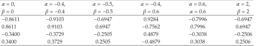
Table 1: The roots ofPnα,βxfor diﬀerent values ofαandβ.

α0, α−0.4, α−0.5, α−0.4, α0.6, α2,

β0 β−0.4 β−0.5 β0.6 α0.6 β2

−0.8611 −0.9103 −0.6947 0.9284 −0.7996 −0.6947

0.8611 0.9103 0.6947 −0.7562 0.7996 0.6947

−0.3400 −0.3729 −0.2505 0.4879 −0.3038 −0.2506

0.3400 0.3729 0.2505 −0.4879 0.3038 0.2506

These polynomials are eigenfunctions of the following singular Sturm-Liouville equa-tion:

1−x2 Φx β−α−βα2xΦx nnβα1Φx 0. 1.3

A consequence of this is that spectral accuracy can be achieved for expansions in Jacobi polynomials so that

Pnα,β1 Γnα

1

n!Γα1 ,

Pnα,β−1

−1nΓnβ1

n!Γβ1 .

1.4

The Jacobi polynomials can be obtained from Rodrigue’s formula as

1−xα1xβPnα,βx −

1ndn

2n_n_!_dxn

1−xαn1xβn. 1.5

Furthermore, we have that

d dx

Pnα,βx

1 2

nαβ1P_nα₋₁1,β1x. 1.6

The Jacobi polynomials are normalized such that

Pnα,β1

nα n

Γnα1

n!Γα1 . 1.7

An important consequence of the symmetry of weight function wx and the orthogonality of Jacobi polynomial is the symmetric relation

(3)

−1 −0.5 0 0.5 1 −1 −0.5 0 0.5 1

−1

−0.8

−0.6

−0.4

−0.2

0 0.2 0.4 0.6 0.8 1

Approximation Exact

−0.015

−0.01

−0.005

0 0.005 0.01 0.015

Error

(a1) (a2)

a

−1 −0.5 0 0.5 1 −1 −0.5 0 0.5 1

−1

−0.8

−0.6

−0.4

−0.2

0 0.2 0.4 0.6 0.8 1

Approximation Exact

Error

−0.04

−0.03

−0.02

−0.01

0 0.01 0.02 0.03 0.04

(b1) (b2)

b

−1 −0.5 0 0.5 1 −1 −0.5 0 0.5 1

−1

−0.8

−0.6

−0.4

−0.2

0 0.2 0.4 0.6 0.8 1

0

Approximation Exact

Error

(c1) (c2)

−0.01

−0.008

−0.006

−0.004

−0.002

0.002 0.004 0.006 0.008 0.01

[image:3.600.130.472.95.683.2]

c

(4)

−1 −0.5 0 0.5 1 −1 −0.5 0 0.5 1

−1

−0.8

−0.6

−0.4

−0.2

0 0.2 0.4 0.6 0.8 1

Approximation Exact

Error −8

−6 −4 −2 0 2 4 6 8

×10−3

(d1) (d2)

d

−0.02

−0.015

−0.01

−0.005

0 0.005

0.01 0.015 0.02

−1 −0.5 0 0.5 1 −1 −0.5 0 0.5 1

−1

−0.8

−0.6

−0.4

−0.2

0 0.2 0.4 0.6 0.8 1

Approximation Exact

Error

(e1) (e2)

e

−1 −0.5 0 0.5 1 −1 −0.5 0 0.5 1

−1

−0.8

−0.6

−0.4

−0.2

0 0.2 0.4 0.6 0.8 1

Approximation Exact

Error

−0.025

−0.02

−0.015

−0.01

−0.005

0 0.005 0.01 0.015 0.02 0.025

(f1) (f2)

[image:4.600.124.474.70.660.2]

f

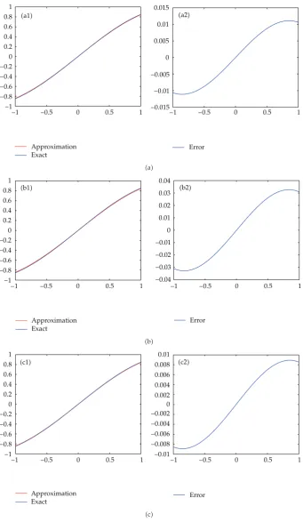
Figure 1: Numerical solution of our example for diﬀerent values ofαandβ.a1α0,β0;a2is error.

(5)

[image:5.600.102.520.112.667.2]

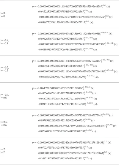
Table 2: The solution of our example for diﬀerent values ofαandβ.

α0,

β0

y−0.00000000000000001119663700028745952445299264438P00,0x 0.91522505937265707954150015923236P10,0x

−0.000000000000000022393274000574919048905985288767P20,0x

−0.059677652961529090927417051547721P₃0,0x.

α−0.4,

β−0.4

y−0.000000000000000009996746174510901192865699495P0−0.4,−0.4x 0.89426538703542076709570198303656P₁−0.4,−0.4x

−0.000000000000000011996095223297443607007612548232P2−0.4,−0.4x

−0.04198983897503790669842860235471P3−0.4,−0.4x.

α−0.5,

β−0.5

y 0.0000000000000000311183604968765645740547197244P0−0.5,−0.5x 0.88795403952304732584548430952028P1−0.5,−0.5x

0.000000000000000031118360496876564574054719724411P2−0.5,−0.5x

−0.036586425139067737724980961913629P3−0.5,−0.5x.

α−0.4,

β0.6

y 0.40613910584685335757685249174382P0−0.4,0.6x 0.48556046784167101822183413097838P1−0.4,0.6x

−0.018735918702094560665272214650799P2−0.4,0.6x

−0.021911869735090742971371812015998P3−0.4,0.6x.

α0.6,

β0.6

y 0.00000000000000000185396073409571348071696317294P00.6,0.6x 0.93795482243803032015459053856673P₁0.6,0.6x

0.0000000000000000059326745972604669042025846148469P20.6,0.6x

−0.078409581597779066879404197800853P30.6,0.6x.

α2,

β2

y 0.000000000000000002334262949979475861874127912143P02,2x 0.97023755744312467875938569010755P12,2x

0.00000000000000001400557769987685517124476747286P22,2x

(6)

[image:6.600.102.499.129.327.2]

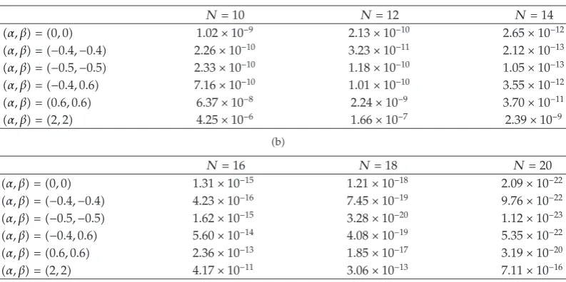
Table 3: Representation of the error by increasing the number of terms in our polynomial solution.

a

N10 N12 N14

α, β 0,0 1.02×10−9 ₂_.₁₃_×₁₀−10 ₂_.₆₅_×₁₀−12

α, β −0.4,−0.4 2.26×10−10 ₃_.₂₃_×₁₀−11 ₂_.₁₂_×₁₀−13 α, β −0.5,−0.5 2.33×10−10 ₁_.₁₈_×₁₀−10 ₁_.₀₅_×₁₀−13 α, β −0.4,0.6 7.16×10−10 ₁_.₀₁_×₁₀−10 ₃_.₅₅_×₁₀−12

α, β 0.6,0.6 6.37×10−8 ₂_.₂₄_×₁₀−9 ₃_.₇₀_×₁₀−11

α, β 2,2 4.25×10−6 ₁_.₆₆_×₁₀−7 ₂_.₃₉_×₁₀−9

b

N16 N18 N20

α, β 0,0 1.31×10−15 ₁_.₂₁_×₁₀−18 ₂_.₀₉_×₁₀−22

α, β −0.4,−0.4 4.23×10−16 ₇_.₄₅_×₁₀−19 ₉_.₇₆_×₁₀−22 α, β −0.5,−0.5 1.62×10−15 ₃_.₂₈_×₁₀−20 ₁_.₁₂_×₁₀−23 α, β −0.4,0.6 5.60×10−14 ₄_.₀₈_×₁₀−19 ₅_.₃₅_×₁₀−22 α, β 0.6,0.6 2.36×10−13 ₁_.₈₅_×₁₀−17 ₃_.₁₉_×₁₀−20

α, β 2,2 4.17×10−11 ₃_.₀₆_×₁₀−13 ₇_.₁₁_×₁₀−16

that is, the Jacobi polynomials are even or odd depending on the order of the polynomial. In this form the polynomials may be generated using the starting form

P₀α,βx 1,

P₁α,βx 1

2

α−β λ1x,

1.9

such that

λαβ1, 1.10

which is obtained from Rodrigue’s formula as follows:

Pnα,βx

1 2n

n

i0

nα i

nβ n−k

1−xn−k1xk. 1.11

Following the two seminal papers of Doha3,4letfxbe an infinitely diﬀerentiable function defined on−1, 1; then we can write

fx

∞

n0

anPnα,βx, 1.12

and, for theqth derivative offx,

fqx

∞

n0

(7)

Then,

aqn 2−q

∞

i0

niqλ−1_qCni,nαq, βq, α, βaniq, ∀n≥0, q≥1, 1.14

where

Cni,nαq, βq, α, β

ni2qλ−1_nnαq1_iΓnλ i!Γ2nλ

× 3F2

⎛

⎝ −i 2ni2qλ nα1 _{; 1}

nqα1 2nλ1

⎞ ⎠_,

mnmm1· · ·mn−1

mn−1!

m−1! .

1.15

For the proof of the above, see3. The formula for the expansion coeﬃcients of a general-order derivative of an infinitely diﬀerentiable function in terms of those of the function is available for expansions in ultraspherical and Jacobi polynomials in Doha 5. Another interesting formula is

xmP_jα,βx

2m

n0

amnjP_jmα,β₋_nx, ∀m, j ≥0, 1.16

with

P₋α,βr x 0, r ≥1, 1.17

where

amnj −1

n₂jm−n_m_!₂_j₂_m₋₂_n_λ_Γ_j_m₋_n_λ_Γ_j_α₁_Γ_j_β₁ Γjm−nα1Γjm−nβ1Γjλ

×

minjm−n,j

max0,j−n

jm−n k

Γjkλ

2k_n_k_j_!_Γ₃_j₂_m₋₂_n₋_k_λ₁

×j−k

i0

−1lΓ2jm−n−k−lα1Γjml−nβ1

l!j−k−l!Γj−lα1Γklβ1

× 2F1

j−k−n, jml−nβ1; 3j2m−2n−kλ1; 2.

1.18

(8)

of boundary value problems 6 and in computational fluid dynamics 7, 8. For the ultraspherical coefficients of the moments of a general-order derivative of an infinitely differentiable function, see5. Collocation method is a kind of spectral method that uses the delta function as a test function. Test functions have an important role because these functions are applied to obtain the minimum value for residual by using inner product. Attention to this point is very important since Tau and collocation methods do not give the best approximation solution of ODEs. Due to adding the boundary conditions, we are forced to eliminate several conditions of orthogonality properties, and this decreases the accuracy of the ODEs solution. Previous explanations do not mean that the accuracy of the collocation method is less than that of the Galerkin method. Many studies on the collocation method have recently appeared in the literature on the numerical solution of boundary value problems9–12. The collocation solution is a piecewise continuous polynomial function. The error has been analyzed for different conditions by different authors. Frank and Ueberhuber13showed equivalence between solutions of collocation method and fixed points of Iterated Defect CorrectionIDeC method. They proved that IDeC method can be regarded as an efficient scheme for solving collocation equations. Ç elik 14,15 investigated the corrected collocation method for the approximate computation of eigenvalues of Sturm-Liouville and periodic Sturm-Liouville problems by a Truncated Chebyshev SeriesTCS. On the other hand, some results on Jacobi approximation were used for analyzing thep-version of finite element method, boundary element method, spectral method for axisymmetrical domain, and various rational spectral methods16–21.

The rest of this paper is organized as follows. In Section 2, the method of solution is developed. InSection 3, we report our numerical findings and demonstrate the accuracy of the proposed scheme by considering a numerical example. Finally, a brief conclusion is presented inSection 4.

2. Jacobi Collocation Method

We consider the class of ODEs with the following form

s

i0

Pixyi l

i0

Qixyi m

i0

RixyiFx, 2.1

wheres, l, m≥0,Pix,Qix,Rix, andFxare defined on the intervala≤x≤b. The most general boundary conditions are

γ0ya γ1ya δ,

α0yb α1yb μ,

2.2

where the real coeﬃcients γi,αi, δ, and μ are appropriate constants and the solution is expressed in the form

y n

r0

crPrα,βx, 2.3

(9)

Any finite rangea≤w ≤bcan be transformed to the basic range−1 ≤x≤1 with the change of variable

w b−ax ba

2 . 2.4

Hence, there is no loss of generality in takinga −1 and b 1. To obtain such a solution, the Jacobi collocation method can be used. Collocation points can be taken as the roots ofPnα,βx 22. Until now we have not the explicit formulas that determine these roots.

Therefore, we use the numerical method to determine these roots, for example, the Newton method. Substituting the Jacobi collocation points in2.1, the following expression can be obtained:

s

i0

Pixj

_n

r0

crPrα,β

xj

i l

i0

Qixj

_n

r0

crPrα,β

xj

i

m i0

Rixj

n

r0

crPrα,β

xj

i

Fxj, j 0,1,2,3, . . . , n.

2.5

The above system of equations constructsn1 nonlinear equations. We impose the boundary conditions to these equations as follows:

γ0

_n

r0

crPrα,βa

γ1

_n

r0

crPrα,βa

δ,

α0

_n

r0

crPrα,βb

α1

_n

r0

crPrα,βb

μ.

2.6

Equations 2.5and 2.6construct then3 nonlinear equations and so we eliminate two equations from 2.1. Thus we have n1 equations and solve this system with Newton iteration method.

3. Illustrative Numerical Example

Consider the following nonlinear boundary value problem:

cosxy2−sin2xy0, 3.1

subject to boundary conditions

y0 0,

yπ

2 1.

(10)

The exact solution isy sinx. We solve it with the above-mentioned methodfor diﬀerent values ofαandβ, and we show the results. We compute the numerical solution for 4 terms inFigure 1.

At first we obtain the roots ofPnα,βx. For this goal we must determine theαandβ

parameters, andTable 1shows the roots.

To apply the method we assume that the solution is in the following form:

y

3

i0

ciP_iα,βx. 3.3

By substitutingyin3.1, we obtain a system of equations, and, with attention to Gaussian nodes, we must solve the set of nonlinear equations. The boundary conditions are imposed on the system of equations with elimination of two equations, and we add these boundary conditions to the system as follows:

cosxj

₃

i0

ciP_iα,βxj

2

−sin2xj

₃

i0

ciP_iα,βxj

0, j 0,1,2,3. 3.4

The above system can be solved with Newton iteration method. We show our results for every parameter as inTable 2. Representation of the error by increasing the number of terms in our polynomial solution is shown inTable 3. It is observable that as the number of terms increases, the absolute error decreases.

4. Conclusion

In this paper, we show that this method is very accurate, even for small value ofni.e.,n4. We see that Chebyshev polynomialthe casesc1andc2and Legendre polynomialthe cases

a1 anda2have not obtained the best approximationsee the caseα −0.4,β 0.6. We

observe that the error is symmetric whenαβsee the casesa2, b2, c2, e2, andf2. When we

increase the number of terms in our computation, we monitor that the error decreases and our computed results are the best.

References

1 G. Szeg, Orthogonal Polynomials, vol. 23, Amer. Math. Soc., 1985.

2 Y. Luke, The Special Functions and Their Approximations, Academic Press, New York, NY, USA, 1969. 3 E. H. Doha, “On the coeﬃcients of diﬀerentiated expansions and derivatives of Jacobi polynomials,”

Journal of Physics. A, vol. 35, no. 15, pp. 3467–3478, 2002.

4 E. H. Doha, “On the construction of recurrence relations for the expansion and connection coeﬃcients in series of Jacobi polynomials,” Journal of Physics. A, vol. 37, no. 3, pp. 657–675, 2004.

5 E. H. Doha, “The ultraspherical coeﬃcients of the moments of a general-order derivative of an infinitely diﬀerentiable function,” Journal of Computational and Applied Mathematics, vol. 89, no. 1, pp. 53–72, 1998.

6 D. Gottlieb and S. A. Orszag, Numerical Analysis of Spectral Methods: Theory and Applications, CBMS-NSF Regional Conference Series in Applied Mathematics, No. 2, SIAM, Philadelphia, Pa, USA, 1977. 7 C. Canuto, M. Y. Hussaini, A. Quarteroni, and T. A. Zang, Spectral Methods in Fluid Dynamics, Springer

(11)

8 R. G. Voigt, D. Gottlieb, and M. Y. Hussaini, Spectral Methods for Partial Diﬀerential Equations, SIAM,

Philadelphia, Pa, USA, 1984.

9 C. de Boor and B. Swartz, “Collocation at Gaussian points,” SIAM Journal on Numerical Analysis, vol. 10, pp. 582–606, 1973.

10 F. A. Oliveira, “Numerical solution of two-point boundary value problems and spline functions,” in

Numerical methods (Third Colloq., Keszthely, 1977), vol. 22 of Colloq. Math. Soc. J´anos Bolyai, pp. 471–490,

North-Holland, Amsterdam, The Netherlands, 1980.

11 R. D. Russell and L. F. Shampine, “A collocation method for boundary value problems,” Numerische

Mathematik, vol. 19, pp. 1–28, 1972.

12 R. Weiss, “The application of implicit Runge-Kutta and collection methods to boundary-value problems,” Mathematics of Computation, vol. 28, pp. 449–464, 1974.

13 R. Frank and C. W. Ueberhuber, “Collocation and iterated defect correction,” in Numerical Treatment

of Diﬀerential Equations, Lecture Notes in Math., Vol. 631, pp. 19–34, Springer, Berlin, Germany, 1978. 14 ˙I. C¸elik, “Approximate calculation of eigenvalues with the method of weighted residuals—collocation

method,” Applied Mathematics and Computation, vol. 160, no. 2, pp. 401–410, 2005.

15 ˙I. C¸elik and G. Gokmen, “Approximate solution of periodic Sturm-Liouville problems with Chebyshev collocation method,” Applied Mathematics and Computation, vol. 170, no. 1, pp. 285–295, 2005.

16 I. Babuˇska and B. Guo, “Direct and inverse approximation theorems for the p-version of the finite element method in the framework of weighted Besov spaces. I. Approximability of functions in the weighted Besov spaces,” SIAM Journal on Numerical Analysis, vol. 39, no. 5, pp. 1512–1538, 2002. 17 I. Babuˇska and B. Guo, “Optimal estimates for lower and upper bounds of approximation errors in

the p-version of the finite element method in two dimensions,” Numerische Mathematik, vol. 85, no. 2, pp. 219–255, 2000.

18 B.-Y. Guo and L. I. Wang, “Jacobi interpolation approximations and their applications to singular diﬀerential equations,” Advances in Computational Mathematics, vol. 14, no. 3, pp. 227–276, 2001. 19 P. Junghanns, “Uniform convergence of approximate methods for Cauchy-type singular integral

equations over-1, 1,” Wissenschaftliche Zeitschrift der Technischen Hochschule Karl-Marx-Stadt, vol. 26, no. 2, pp. 251–256, 1984.

20 E. P. Stephan and M. Suri, “On the convergence of the p-version of the boundary element Galerkin method,” Mathematics of Computation, vol. 52, no. 185, pp. 31–48, 1989.

21 Z.-Q. Wang and B.-Y. Guo, “A rational approximation and its applications to nonlinear partial diﬀerential equations on the whole line,” Journal of Mathematical Analysis and Applications, vol. 274, no. 1, pp. 374–403, 2002.

22 ˙I. C¸elik, “Collocation method and residual correction using Chebyshev series,” Applied Mathematics

(12)

Submit your manuscripts at

http://www.hindawi.com

Hindawi Publishing Corporation

http://www.hindawi.com Volume 2014

Mathematics

Journal of

http://www.hindawi.com Volume 2014 Mathematical Problems in Engineering

Hindawi Publishing Corporation http://www.hindawi.com

Differential Equations International Journal of

Volume 2014

Applied MathematicsJournal of

Probability and Statistics Hindawi Publishing Corporation

http://www.hindawi.com Volume 2014 Journal of

Mathematical PhysicsAdvances in

Complex Analysis

Journal of

Optimization

Journal of

Combinatorics

International Journal of

http://www.hindawi.com Volume 2014 Operations ResearchAdvances in

Journal of

Function Spaces

Abstract and Applied Analysis Hindawi Publishing Corporation

International Journal of Mathematics and Mathematical Sciences

Hindawi Publishing Corporation http://www.hindawi.com Volume 2014

The Scientific

World Journal

Algebra

Discrete Dynamics in Nature and Society

Decision Sciences

Advances in

Discrete Mathematics

Journal of