IMAGE COMPRESSION USING WAVELETS

GE-International Journal of Engineering Research

Vol. 4, Issue 5, May 2016 IF- 4.721 ISSN: (2321-1717)

© Associated Asia Research Foundation (AARF) Publication

Website: www.aarf.asiaEmail : [email protected] , [email protected]

IMAGE COMPRESSION USING WAVELETS

1

Prof.C.Arunabala 2Suneetha 1

Electronics and communications engineering, Ravindra College of Engineering For Women,Kurnool-3-AP-INDIA.

2

Electronics and communications engineering, Kallam Haranadhreddy Institute of Technology, Guntur-AP-INDIA.

ABSTRACT

Signal analysts already have at their disposal an impressive arsenal of tools. Perhaps

the most well-known of these is Fourier analysis, which breaks down a signal into constituent

sinusoids of different frequencies. Another way to think of Fourier analysis is as a

mathematical technique for transforming our view of the signal from time-based to

frequency-based. For many signals, Fourier analysis is extremely useful because the signal’s

frequency content is of great importance. Fourier analysis has a serious drawback. In

transforming to the frequency domain, time information is lost. When looking at a Fourier

transform of a signal, it is impossible to tell when a particular event took place. If the signal

properties do not change much over time — that is, if it is what is called a stationary signal—

this drawback isn’t very important. However, most interesting signals contain numerous non

stationary or transitory characteristics: drift, trends, abrupt changes, and beginnings and

ends of events. These characteristics are often the most important part of the signal, and

Fourier analysis is not suited to detecting them. In an effort to correct this deficiency, Dennis

Gabor (1946) adapted the Fourier transform to analyze only a small section of the signal at a

time—a technique called windowing the signal. Gabor’s adaptation, called the Short-Time

Fourier Transform (STFT), maps a signal into a two-dimensional function of time and

frequency.The STFT represents a sort of compromise between the time- and frequency-based

signal event occurs. However, you can only obtain this information with limited precision,

and that precision is determined by the size of the window. While the STFT compromise

between time and frequency information can be useful, the drawback is that once you choose

a particular size for the time window, that window is the same for all frequencies. Many

signals require a more flexible approach—one where we can vary the window size to

determine more accurately either time or frequency.

Keywords

COMPRESSION AND DECOMPRESSION TECHNIQUES ,WAVELETS, DIGITIZATION ,QUANTIZATION ,ENTROPY CODING

Introduction

COMPRESSION AND DECOMPRESSION TECHNIQUES:

One of the imports aspects of image storage is its efficient Compression. To make this fact

clear let's see an example. An image, 1024 pixel x 1024 pixel x 24 bit without compression would require 3 MB of storage and 7 minutes for transmission, utilizing a high speed 64

Kbits/s ISDN line. If the image is compressed at a 10:1 compression ratio, the storage

requirement is reduced to 300 KB and the transmission time drops to under 6 seconds. Seven

1 MB images can be compressed and transferred to a floppy disk in less time than it takes to

send one of the original files, uncompressed, over an AppleTalk network. In a distributed

environment large image files remain a major bottleneck within systems. Compression is an

important component of the solutions available for creating file sizes of manageable and

transmittable dimensions. Increasing the bandwidth is another method, but the cost

sometimes makes this a less attractive solution.. Platform portability and performance are

important in the selection of the compression/decompression technique to be employed.

Compression solutions today are more portable due to the change from proprietary high end

solutions to accepted and implemented international standards. JPEG is evolving as the

industry standard technique for the compression of continuous tone images.

Image Compression Using Wavelets:

Images require much storage space, large transmission bandwidth and long transmission time. The only way currently to improve on these resource requirements is to compress

images, such that they can be transmitted quicker and then decompressed by the receiver. In

image processing there are 256 intensity levels (scales) of grey. 0 is black and 255 is white.

11111111. An image can therefore be thought of as grid of pixels, where each pixel can be

represented by the 8-bit binary value for grey-scale. The resolution of an image is the pixels

per square inch. (So 500dpi means that a pixel is 1/500th of an inch). To digitize a one-inch

square image at 500 dpi requires 8 x 500 x500 = 2 million storage bits. Using this

representation it is clear that image data compression is a great advantage if many images are

to be stored, transmitted or processed. "Image compression algorithms aim to remove

redundancy in data in a way which makes image reconstruction possible." By removing the

redundant data, the image can be represented in a smaller number of bits, and hence can be

compressed.

With the growth of technology and the entrance into the Digital Age, the world has found

itself amid a vast amount of information. Dealing with such enormous amount of information

can often present difficulties. Digital information must be stored and retrieved in an efficient

manner, in order for it to be put to practical use. Wavelet compression is one way to deal with

this problem. For example, the FBI uses wavelet compression to help store and retrieve its

fingerprint files. The FBI possesses over 25 million cards, each containing 10 fingerprint

impressions. To store all of the cards would require over 250 terabytes of space. Without

some sort of compression, sorting, storing, and searching for data would be nearly

impossible. Using wavelets, the FBI obtains a compression ratio of about 1:20.

COMPRESSION STEPS

The steps needed to compress an image are as follows:

1. Digitize the source image into a signal s, which is a string of numbers.

2. Decompose the signal into a sequence of wavelet coefficients w.

3. Use thresholding to modify the wavelet coefficients from w to another sequence w'.

4. Use quantization to convert w' to a sequence q.

DIGITIZATION

The first step in the wavelet compression process is to digitize the image. The digitized image

can be characterized by its intensity levels, or scales of gray which range from 0 (black) to

255 (white), and its resolution, or how many pixels per square inch. Each of the bits involved

in creating an image takes up both time and money, so a tradeoff must be made.

WAVELET DECOMPOSITION:

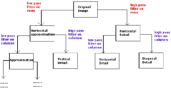
Images are treated as two dimensional signals, they change horizontally and vertically, thus

2D wavelet analysis must be used for images. 2D wavelet analysis uses the same ’mother wavelets’ but requires an extra step at every level of decomposition. The 1D analysis filtered

out the high frequency information from the low frequency information at every level of

decomposition; so only two sub signals were produced at each level. In 2D, the images are

considered to be matrices with N rows and M columns. At every level of decomposition the

horizontal data is filtered, then the approximation and details produced from this are filtered

on columns. At every level, four sub-images are obtained; the approximation, the vertical

detail, the horizontal detail and the diagonal detail. Below the Saturn image has been

decomposed to one level. The wavelet analysis has found how the image changes vertically,

horizontally and diagonally.

Fig 2:2-D Decomposition of Saturn Image to level 1

To get the next level of decomposition the approximation sub-image is decomposed, this idea

can be seen in figure 3. When compressing with orthogonal wavelets the energy retained is:

The number of zeros in percentage is defined by:

Fig 3: Saturn Image decomposed to Level 3. Only the 9 detail images and the final

THRESHOLDING

In certain signals, many of the wavelet coefficients are close or equal to zero.

Through a method called thresholding, these coefficients may be modified so that the

sequence of wavelet coefficients contains long strings of zeros. Through a type of

compression known as entropy coding, these long strings may be stored and sent

electronically in much less space.

QUANTIZATION

The fourth step of the process, known as quantization, converts a sequence of

floating numbers w' to a sequence of integers q. The simplest form is to round to the nearest

integer. Another option is to multiply each number in w' by a constant k, and then round to

the nearest integer. Quantization is called lossy because it introduces error into the process,

since the conversion of w' to q is not a one-to-one function.

ENTROPY CODING

Wavelets and thresholding help process the signal, but up until this point, no

compression has yet occurred. One method to compress the data is Huffman entropy coding.

With this method, and integer sequence, q, is changed into a shorter sequence, e, with the

numbers in e being 8 bit integers. The conversion is made by an entropy coding table.

Strings of zeros are coded by the numbers 1 through 100, 105, and 106, while the non-zero

integers in q are coded by 101 through 104 and 107 through 254. In Huffman entropy coding,

the idea is to use two or three numbers for coding, with the first being a signal that a large

number or long zero sequence is coming. Entropy coding is designed so that the numbers that

are expected to appear the most often in q, need the least amount of space in e.

Conclusion

Results:

The results of the compression achieved were as follows.

Image:

Original Image Size: 66kb (Bitmap)

Compressed Image Size (using WinZip): 54kb

Sound:

Original File Size : 215kb (wave)

Compressed File Size(using WinZip): 196kb

Compressed File Size (using Wavelets and then WinZip): 26kb

Original Gray Level Image:

Compressed Image (Using Bi-Orthogonal 3.7 Decomposition Level 2):

Matlab Code:

%to compress an image

function Compress(FileName) % calling a function

[ImgData,Map] = imread(FileName); % read the image and store the values in an array

[Coef,Pos] = wavedec2(ImgData,2,'Bior3.7'); % apply wavelet decomposition

%[thr,s_or_h,keep_app] = ddencmp('cmp','wv',ImgData);

[thr,s_or_h,keep_app] = compthreshold(c,s,percentageCompression,keepapp); apply

[xcomp,CXC,LXC,PERF0,PERFL2] =

wdencmp('gbl',Coef,Pos,'Bior3.7',2,thr,s_or_h,keep_app);

MaxValue = max(CXC);

NormalizationFactor = MaxValue / 255; %calculate normalization factor

NormalizedCoef = Coef / NormalizationFactor; % calculate normalization coefficient

IntValues = fix(NormalizedCoef);

EightBitValues = uint8(IntValues); Convert into 8 bit data

save compressed.mat EightBitValues Pos NormalizationFactor Map;

% save the compressed image

%%%%% applying the thresholding values

function [threshold,sorh,keepap] = compthreshold(c,s,percentage,keepapp)

sorh = 'h'; % type of compression hard which uses averaging filtering

keepap = keepapp;

if keepapp == 1

x = abs (c(prod(s(1,:))+1:end)); calculate the threshold for a given image

x = sort(x);

dropindex = length(x) * percentage/100;

dropindex = round(dropindex);

threshold = x(dropindex); initialize the value as a threshold

else %drop coefficients even from the approximation

x = abs(c);

x = sort(x);

dropindex = length(x) * percentage/100;

dropindex = round(dropindex);

threshold = x(dropindex);

if (threshold == 0) % if the value of threshold is 0 then execute the following statement

threshold = 0.05*max(abs(x));

end

%now apply the above two functions for the image compression

function y = ImageCompression (levelOfdecomposition,percentageCompression,keepapp)

%[X,map] = imread ('badcloning','jpg'); % read the image and store the data into an array

load wbarb; %here loading a wbarb image from image processing toolbox of matlab

IMWRITE(X,map,'OriginalImage.bmp');

figure;

colormap(map); %apply the mapping

image(X);

save Original.mat X; %save the read image

title('ORIGINAL IMAGE');

[c,s] = wavedec2(X,levelOfdecomposition,'bior3.7');%apply wavlet decomposition

[threshold,sorh,keepapp] = compthreshold(c,s,percentageCompression,keepapp);

[Xcomp,cxc,lxc,perf0,perfl2] = wdencmp

('gbl',c,s,'bior3.7',levelOfdecomposition,threshold,sorh,keepapp);

save Compressed.mat cxc;

IMWRITE(Xcomp,map,'compressedImage.bmp');

figure;

%colormap(map);

colormap(map);

image(Xcomp);

title('COMPRESSED IMAGE');

%%%%

%% apply two dimensional wavlet transforms

function TwoDimDWT

ImgData = imread('cons.bmp');

[a1,h1,v1,d1] = dwt2(ImgData,'Bior3.7'); %educe it into decomposition levels

figure;

image(ImgData);

title('Original Image');

colormap(map);

pause;

subplot(221);

image(a1);

title('Approximations');

subplot(222);

image(h1);

title('Horizontal Details');

subplot(223);

image(v1);

title('Vertical Details');

subplot(224);

image(d1);

title('Diagonal Details');

ReConsImg = idwt2(a1,h1,v1,d1,'Bior3.7'); %reconstruct the image by apllying inverse

transforms

pause;

subplot(111);

image(ReConsImg);

colormap(map);

title('Re-Constructed Image');

%%%%%

%% now uncompress the image

function Uncompress

load compressed.mat;% load the previously saved compressed image and apply inverse

transforms

ActualCoef = double(EightBitValues); %convert back into original bits back from 8-bit data

ActualCoef = ActualCoef .* NormalizationFactor; %calculate actual coefficients

imwrite(ImgData,Map,'aRecon.bmp'); %write the uncompressed image

APPLICATIONS:

Applications of image processing:

1.Photography and printing

2.Satellite image processing

3. Medical image processing

4. Face detection, feature detection, face identification

5. Microscope image processing

References

[1] Digital Image Processing using MATLAB--Rafael C. Gonzalez, Richard E. Woods

Steven C. Eddies

[2] Guttmann, Peter (1995)-- Introduction to Data Compression.

[3] Lane, Tom (1995)--Introduction to JPEG. Compression.

[4] http://www.cis.ohio-state.edu/hypertext/faq/usenet/compression-faq/part2/faq.html

[5] Sprigg, Graham (ed.) (1995)-- The Unsolved Problem of Image Compression.

[6] Wavelet Toolbox, Signal Processing toolbox, Symbolic toolbox.

[7] Burt, P.; Adelson, E. (1 April 1983). "The Laplacian Pyramid as a Compact Image

Code".IEEE Transactions on Communications31(4): 532–

540. doi:10.1109/TCOM.1983.1095851.

[8]Jump up^ Shao, Dan; Kropatsch, Walter G. (February 3–5, 2010). "Irregular Laplacian

Graph Pyramid" (PDF).Computer Vision Winter Workshop 2010(Nove Hrady, Czech