A constraint based random search algorithm for optimizing neural network architectures and ensemble construction in detecting loss of coolant accidents in nuclear power plants

Citation:

Tian, D and Deng, J and Vinod, G and Santhosh, TV (2019) A constraint-based random search

algorithm for optimizing neural network architectures and ensemble construction in detecting

loss of coolant accidents in nuclear power plants.

In: 2018 11th International Conference on

Developments in eSystems Engineering (DeSE), 2nd – 5th September 2018, Cambridge. DOI:

https://doi.org/10.1109/DeSE.2018.00036

Link to Leeds Beckett Repository record:

http://eprints.leedsbeckett.ac.uk/5845/

Document Version:

Conference or Workshop Item

The aim of the Leeds Beckett Repository is to provide open access to our research, as required by

funder policies and permitted by publishers and copyright law.

The Leeds Beckett repository holds a wide range of publications, each of which has been

checked for copyright and the relevant embargo period has been applied by the Research Services

team.

We operate on a standard take-down policy.

If you are the author or publisher of an output

and you would like it removed from the repository, please

contact us

and we will investigate on a

case-by-case basis.

A Constraint-based Random Search Algorithm for

Optimizing Neural Network Architectures and

Ensemble Construction in Detecting Loss of

Coolant Accidents in Nuclear Power Plants

David Tian Leeds Beckett University

Leeds, UK [email protected]

T.V. Santhosh Bhabha Atomic Research Centre

Mumbai, India [email protected]

Jiamei Deng Leeds Beckett University

Leeds, UK [email protected]

Gopika Vinod

Bhabha Atomic Research Centre Mumbai, India

[email protected]

Abstract— One major accident of a nuclear power plant (NPP) is the loss of a coolant accident (LOCA) which is caused by a large break in an inlet header (IH) of a nuclear reactor. This work proposes a constraint-based random search algorithm for optimizing neural network (NN) architectures and ensemble construction in three stages for detecting the break size of an IH of a NPP. In stage one, a number of 2-hidden layer, 3-hidden layer and 4-hiddden layer network architectures are created using a proposed constraint satisfaction algorithm. Then, an optimised 2-hidden layer network, an optimised 3-hidden layer network and an optimised 4-hidden layer network are chosen from these architectures by training and testing them on a transient dataset of IHs and a linear interpolation dataset. In stage two, the optimised 2-hidden layer network, the optimised 3-hidden layer network and the optimised 4-hidden layer network are trained and tested iteratively 200 times on the transient dataset to further improve their performance. In stage three, the optimised 2-hidden layer network, the optimised 3-hidden layer network and the optimised 4-3-hidden layer network are combined into a neural network ensemble (NNE) using a weighted meaning approach. The results show that the NNE outperformed the individual optimised neural networks in detecting the break size of an IH.

Keywords—Neural Networks, Constraint Satisfaction, Neural Network Ensemble, Loss of Coolant Accidents, Linear Interpolation

I. INTRODUCTION

Nuclear power plants (NPP) life management is concerned with monitoring the safety and the conditions of the components of a NPP and the maintenance of the NPP in order to extend its lifetime. It is crucial to regularly monitor the safety of the components of a NPP to detect as early as possible any serious anomalies which would potentially cause accidents. When an accident is predicted to occur or occurring, the plant operator must take necessary actions as quickly as possible to safeguard the NPP, which involves complex judgements, making trade-offs between demands and requires a lot of expertise to make critical decisions. It is commonly believed that timely and correct decisions in these

situations could either prevent an event from developing into a severe accident or mitigate the undesired consequences of an accident. As NPPs become more advanced, their safety monitoring approaches grow considerably. Current approaches include nuclear reactor simulators, safety margin analysis [15], Probabilistic Safety Assessment (PSA) [15] and artificial intelligence (AI) methods such as neural networks [5-8]. Nuclear reactor simulators such as RELAP5-3D [4] simulate the dynamics of a NPP in accidental scenarios and generate transient datasets of reactors. Safety margin analysis analyses the values of the safety parameters of a reactor and triggers an alert to the plant operator if the safety margin falls below a minimum safety margin. PSA computes the probability of occurrence of accidents based on the probabilities of the component failures which cause the accidents. These approaches are often used to together to safeguard NPPs. Na MG et al [1] generated transient data of IHs using MAAP4 code and trained neural networks on the transient data to detect LOCA in an advanced power reactor 1400 (APR1400). Zio E et al [11] applied fuzzy similarity analysis approaches to detecting the failure modes of nuclear systems. Souza et al [12] developed a RBF network capable of online identifying the accidental dropping of the control rod at the reactor core of a pressurised water reactor. Wei X et al [13] developed self-organizing radial basis function (RBF) networks to predict fuel rod failure of nuclear reactors. Santhosh et al [3] trained a neural network on a transient dataset generated using RELAP5-3D to detect the size of a break, the location of the break in the PHT with the availability of the emergency core cooling system (ECCS) which automatically shuts down the reactor to prevent a subsequent accident.

of its search space. To improve the efficiency of solving a CSP, the CSP can be reduced to a simpler equivalent CSP with a smaller size of the search space by achieving the arc-consistency of the CSP using the AC-3 algorithm [18]. CS has been successfully applied to different problems such as tasks scheduling and resource optimization.

The objective of this work is to propose a random search algorithm based on constraint satisfaction to optimize multilayer perceptron (MLP) architectures and to construct a neural network ensemble to identify break sizes of inlet headers (IHs) of a Pressurized Heavy Water Reactor (PHWR) [2, 3]. This paper is organized as follows. Section 2 describes the LOCA of a PHWR and the generation of a transient dataset using RELAP5-3D; Section 3 proposes the constraint-based random search algorithm; Section 4 presents the results of applying the proposed methodology to LOCA detection; Section 5 discusses the results; conclusions and future work are presented in Section 6.

II. LOSS OF COOLANT ACCIDENTS OF A PHWR This work used RELAP5-3D to simulate the dynamics of the parameters of a PHWR in LOCA scenarios and generate a transient dataset for training neural networks to detect the break sizes of the IHs during LOCA scenarios. A LOCA is caused by a large break of the IHs of the primary heat transport system (PHT) (Fig. 1) of a PHWR as follows. When large breaks of inlet headers of the PHT occur, the system depressurizes rapidly which causes coolant voiding into the reactor core. This coolant voiding into the core causes positive reactivity addition and consequent power rise. Then, the emergency core cooling system automatically shuts down the reactor to keep the NPP safe. When a break occurs, transient data such as the temperature and pressure of the IHs can be collected during a short time period to detect the size of the break using neural networks. The break size is defined as the percentage of the cross-sectional area of an IH. The break size is between 0% (no break) and 200% i.e. double

Fig. 1: The PHT of a PHWR [2]

cross-sectional areas of an IH (a complete rupture of the IH). It is infeasible to generate all possible break sizes. In this study, a transient dataset consisting of the 10 break sizes 0%, 20%, 40%, 50%, 60%, 75%, 100%, 120%, 160% and 200% was generated using RELAP5-3D. The break sizes of 20% or greater are considered as large breaks. For each break size, the 37 signals used by Santhosh et al [3] were collected at various parts of the PHT over 60 seconds using RELAP5-3D under the assumption that this time duration is sufficient to identify LOCA. The 37 signals are measurements of the flow rate, the temperatures and the pressures of the various parts of the PHT. For each break size, the signals were measured at 541 time instants within a 60s duration. Each break size class of the transient dataset consists of 541 instances (observations) and 37 features (signals). The transient dataset is a 5410×38 matrix with the last column representing the break size (the target).

III. THE CONSTRAINT-BASED RANDOM SEARCH ALGORITHM

The proposed algorithm consists of 3 stages (Fig. 2). In the 1st _{stage, a number of 2-hidden layer, 3-hidden layer and}

4-hiddden layer network architectures are created using a proposed constraint satisfaction algorithm called random walk heuristic. Then, an optimised 2-hidden layer network, an optimised 3-hidden layer network and an optimised 4-hidden layer network are chosen from these architectures by training and testing the architectures on the transient dataset and a linear interpolation dataset containing the break sizes not present in the transient dataset. Linear interpolation [9] is a method of constructing new data points within the range of a set of known data points by fitting straight lines using linear polynomials. The break sizes 2.5%, 5%, 7.5%, 10%, 12.5%,…,195% and 197.5% which are missing in the transient dataset, are generated using linear interpolation. For each missing break size, 541 instances are generated giving a total of 38411 instances. The transient dataset and the dataset generated by linear interpolation are merged into a new dataset D containing 43821 instances. D is randomly split into a 50% training set, a 25% validation set and a 25% test set using the random sub-sampling with no replacement method [10].

Thereafter, the 2-hidden layer, 3-hidden layer and 4-hiddden layer network architectures are trained and tested to select an optimized 2-hidden layer architecture, an optimized 3-hidden layer architecture and an optimised 4-hidden layer architecture. The 37 inputs and the break size targets of the training set are rescaled to the interval [-1,1] using min-max normalization before training the neural networks. When testing the trained networks, the outputs of the networks for the test set are transformed back to the target break size range [0%, 200%] by inversing the min-max normalization calculation. The Levenberg-Marquardt algorithm [7, 8] of Matlab 2017b is used for networks training with the maximum epochs set to 1000 and the learning rate set to 0.001.

In the 2nd _{stage, the optimised 2-hidden layer network, the}

optimised 3-hidden layer network and the optimised 4-hidden layer network are trained and tested iteratively 200 times on the transient dataset respectively to further improve their performance. In stage three, the optimised 2-hidden layer network, the optimised 3-hidden layer network and the optimised 4-hidden layer network are combined into a neural network ensemble (NNE) using a weighted meaning approach [19].

The following performance measures are used to evaluate the performances of the neural networks in detecting LOCA:

 The root mean square error (RMSE) of a break size k:

𝑅𝑀𝑆𝐸𝐾 = √𝑀𝑆𝐸𝐾 (1) and

𝑀𝑆𝐸𝐾 =

∑𝑀𝑖=1(𝑂𝑖−𝑇𝑖)2

𝑀 (2)

where M is the number of the patterns of break size k in the test set; i is the ith _{pattern of break size k in the test}

set; 𝑂𝑖 is the output of the network for the ith _{pattern; 𝑇}

𝑖

is the break size target of the ith _pattern.  𝑀𝑒𝑎𝑛 𝑅𝑀𝑆𝐸

=

∑𝐾𝑅𝑀𝑆𝐸𝐾

N

(3)

where N is the number of the different break sizes in the test set; in this study, N=10 (10 break sizes). The RMSE of a break size measures the performance of a network in detecting that specific break size. The mean RMES measures the average performance of a network in detecting break sizes.

A. Creating Neural Network Architectures using Constraint Satisfaction (Stage 1)

In [18], a CSP is defined as a triple (Z,D,C) where Z is a finite set of variables; D is the set of the domains of the variables and C is a set of constraints on subsets of the variables. A label is a variable-value pair which represents the assignment of the value to the variable. The label <x,v> denotes assigning the value v to the variable x.

Constraint satisfaction can be used to generate network architectures whose numbers of inputs, numbers of neurons of a hidden layer, and numbers of weights are bounded by user-specified upper and lower limits. The upper and lower limits can be specified based on the user´s prior knowledge about network architectures with high performances. Then, the problem of creating a 2-hidden layer architecture (H1,H2) can be modelled as a CSP CSP_MLP:

CSP_MLP

Variables: H1, H2; Domains of H1 and H2:

D(H1)={mini_neu,mini_neu+1,…,max_neu}; D(H2)={mini_neu,mini_neu+1,…,max_neu}; Constraint 1 (C1): S×H1 + H1×H2 + H2 ≥ min_ws; Constraint 2 (C2): S×H1 + H1×H2 + H2 ≤ max_ws; Constraint 3 (C3): H1 > H2;

where H1 is the number of the neurons of the 1st hidden layer; H2 is the number of the neurons of the 2nd hidden layer; min_ws and max_ws are the lower and the upper bounds on the number of weights of an architecture; S is the number of inputs; min_neu and max_neu are the minimum and the maximum number of neurons of a hidden layer. A CSP_MLP consists of H1, H2, D(H1), D(H2), C1, C2 and C3. C1 constrains the number of the weights of an architecture to be at least min_ws; C2 constrains the number of the weights of an architecture to be at most max_ws. An assignment of values to H1 and H2 satisfying C1 and C2 is a solution of CSP_MLP. For example, with the settings: S=15, min_neurons=5, max_ neurons=40, ws_min=490 and ws_max=510, C1 becomes 15×H1+H1×H2+H2 ≥ 490 and C2 becomes 15×H1+H1×H2+H2 ≤ 510. A solution of CSP_MLP is the vector (21,8) which corresponds to a network architecture with 15 inputs, 21 neurons in the 1st hidden layer, 8 neurons in the 2nd hidden layer and 1 output neuron. To create a 3-hidden layer architecture (H1,H2, H3), a CSP_MLP2 is solved where H3 is the number of the neurons in the 3rd _{hidden layer:}

CSP_MLP2

Variables: H1, H2, H3; Domains of H1, H2 and H3:

D(H1)={mini_neu,mini_neu+1,…,max_neu}; D(H2)={mini_neu,mini_neu+1,…,max_neu}; D(H3)={mini_neu,mini_neu+1,…,max_neu};

Constraint 4 (C4): S×H1 + H1×H2 + H2×H3+H3 ≥ min_ws; Constraint 5 (C5): S×H1 + H1×H2 + H2×H3+H3 ≤

max_ws;

To create a 4-hidden layer architecture (H1,H2, H3, H4), a CSP_MLP3 is solved where H4 is the number of the neurons in the 4th _{hidden layer:}

CSP_MLP3

Variables: H1, H2, H3, H4; Domains of H1, H2, H3 and H4:

D(H1)={mini_neu,mini_neu+1,…,max_neu}; D(H2)={mini_neu,mini_neu+1,…,max_neu}; D(H3)={mini_neu,mini_neu+1,…,max_neu}; D(H4)={mini_neu,mini_neu+1,…,max_neu};

Constraint 6 (C6): S×H1 + H1×H2 + H2×H3+H3×H4+H4 ≥ min_ws;

1

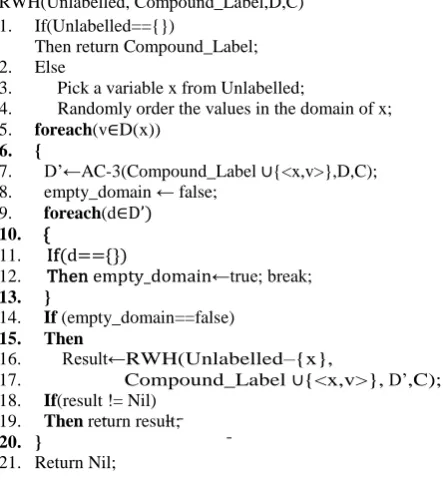
[image:5.595.317.555.64.244.2]

A random walk heuristic (RWH) (Fig. 3) is proposed to find a solution to a CSP_MLP or CSP_MLP2 or CSP_MLP3. The search space of CSP_MLP can be represented as a tree where each node represents a variable with the root node at top of the tree; each branch represents an assignment of a value in the domain of a variable to that variable and each leaf (a bottom node) represents a solution candidate. To solve CSP_MLP, the RWH assigns a random value v1 to H1 and looks ahead whether this partial solution candidate (v1,H2) leads to a solution of CSP_MLP without both assigning a value v2 to H2 and checking the satisfiability of C1 and C2 of the solution candidate (v1,v2). If (v1,H2) does not lead to a solution, a new value v’ is assigned to H1 repeatedly until a partial solution candidate (v’,H2) leads to a solution (v’,v2) (Fig. 4).

Algorithm 1: Random walk heuristic Input: a CSP

Output: S, a solution or Nil if no solution exists 1. S← RWH(Z,{},D,C); /* CSP=(Z,D,C) */ 2. Return S;

RWH(Unlabelled, Compound_Label,D,C) 1. If(Unlabelled=={})

Then return Compound_Label; 2. Else

3. Pick a variable x from Unlabelled;

4. Randomly order the values in the domain of x; 5. foreach(v∈D(x))

6. {

7. D’←AC-3(Compound_Label ∪{<x,v>},D,C); 8. empty_domain ← false;

9. foreach(d∈D’) 10. {

11. If(d=={})

12. Then empty_domain←true; break;

13. }

14. If (empty_domain==false) 15. Then

16. Result←RWH(Unlabelled–{x},

17. Compound_Label ∪{<x,v>}, D’,C); 18. If(result != Nil)

19. Then return result; 20. }

21. Return Nil;

Fig. 3: Pseudocode of the random walk heuristic

[image:5.595.46.268.306.547.2]

In Fig. 4, the arrows indicate the order of traversal of the complete search space. When min_neu or min_neu+1 is assigned to H1, AC-3 reduces D(H2) to an emptyset; when min_neu+2 is assigned to H1, AC-3 reduces D(H2) to {max_neu-2, max_neu-1,max_ neu} and a solution (min_neu+2,max_neu-2) is found by assigning max_neu-2 to H2. When a value is assigned to H1, a look-ahead operation is performed by calling the AC-3 algorithm [22] (step 7 of the RWH procedure) which reduces the CSP_MLP to a simpler CSP with smaller domain sizes for the variables. Redundant values of a variable are the values which violate the constraints on that variable. AC-3 maintains the arc-consistency of a CSP by removing any redundant values from

Fig. 4: The search space exploration of random walk heuristic for solving CSP_MLP.

the domains of the variables of the CSP. An arc-consistent CSP is returned by AC-3. In [22], the arc-consistency of a CSP is defined as follows:

 A variable X is arc-consistent with another variable Y if, for every value a in the domain of X there exists a value b in the domain of Y such that (a,b) satisfies all the constraints between X and Y.

 A CSP is arc-consistent if every variable is arc-consistent with every other one.

If AC-3 reduces the domain of H1 or that of H2 to an empty set, there is no compatible value in D(H1) or D(H2) which satisfies C1 and C2, so there is no solution to the CSP. The worst case computational complexity of AC-3 is O(𝑒𝑑3_{) [22]}

where e is the number of constraints and d is the size of the largest domain of the variables. In the worst case, AC-3 (step 7 of RWH) is called d times for each variable. Therefore, the worst case computational complexity of Algorithm 1 is O(𝑒𝑑4_{𝑛) where n is the total number of variables in the CSP.}

To find an optimised 2-hidden layer architecture, a number of 2-hidden layer architectures are generated by solving CSP_MLPs using the RWH which was implemented using the ECLiPSe constraint logic programming language [20]. To find an optimised hidden layer architecture, a number of 3-hidden layer architectures are generated by solving CSP_MLP2s. To find an optimised 4-hidden layer architecture, a number of 4-hidden layer architectures are generated by solving CSP_MLP3s.

B. Optimizing the Weights of the Optimised Architectures by Iterative Training and Testing (Stage 2)

minimum point in the local region of the minimum point of the last iteration. The optimised network among the K networks is obtained after K iterations of the training-testing process. The iterative training-testing procedure is applied to the optimised 3-hidden layer architecture and the optimised 4-hidden layer architecture respectively to further optimize the weights of the architectures.

Algorithm 2: Iterative training-testing procedure Input: a MLP, transient data, K (iterations) Output: optimised MLP

1. net ← a MLP;

2. optimised_net ← net;

3. t ←1;

4. for (t ≤ K) {

5. Randomly split transient data into a 50% training set, a 25% validation set and a 25% test set;

6. Set the initial weights of the training algorithm to the weights of net;

7. net ← train(net,train_set,valid_set);

8. mean_rmse ← test(net,test_set);

9. If (mean_rmse < mean_rmse of optimised_net)

10. Then optimised_net ← net;

11. t←t+1;

12. }

13. Output optimised_net;

Fig. 5: The iterative training and testing procedure

C. Creating a Neural Network Ensemble from the Optimised Networks (Stage 3)

The outputs of the optimised 2-hidden layer, 3-hidden layer and 4-hidden layer networks are combined together to make a NNE using the weighted mean approach [19] to make a prediction on unseen data. The output 𝐹(𝑥𝑖) of the

ensemble for an unseen pattern 𝑥𝑖 is computed as the weighted sum of the models’ outputs:

𝐹(𝑥𝑖) = ∑𝑛𝑗=1𝑤𝑗∙ 𝑓𝑗(𝑥𝑖) (4)

where 𝑓𝑗(𝑥𝑖) is the output of model j; n is the number of

models; each weight 𝑤𝑗is related to the mean RMSE of model

j on the test set:

𝑤𝑗 =

𝑎𝑑𝑗𝑢𝑠𝑡𝑒𝑑 𝑚𝑒𝑎𝑛 𝑅𝑀𝑆𝐸_𝑗

∑𝑛_𝑘=1𝑎𝑑𝑗𝑢𝑠𝑡𝑒𝑑 𝑚𝑒𝑎𝑛 𝑅𝑀𝑆𝐸_𝑘 (5)

where adjusted mean 𝑅𝑀𝑆𝐸𝑗 is determined by:

adjusted_mean_𝑅𝑀𝑆𝐸𝑗= 1- average mean 𝑅𝑀𝑆𝐸𝑗 (6)

where the average mean 𝑅𝑀𝑆𝐸𝑗is determined by: 𝑎𝑣𝑒𝑟𝑎𝑔𝑒_𝑚𝑒𝑎𝑛_𝑅𝑀𝑆𝐸𝑗= _∑ 𝑚𝑒𝑎𝑛 𝑅𝑀𝑆𝐸𝑗

𝑚𝑒𝑎𝑛 𝑅𝑀𝑆𝐸𝑘 𝑛

𝑘=1

(7) where mean 𝑅𝑀𝑆𝐸𝑗 is the mean RMSE of model j on the test

set.

IV. RESULTS

A. The Optimised Network Architectures (Stage 1)

Our prior knowledge about network architectures with high performances in detecting LOCA of NPPs is that the

maximum number of weights is less than N/2 where N is the size of the training set; the number S of inputs is 37; the number of neurons of each hidden layer is between 5 and 40. The parameters of CSP_MLP, CSP_MLP2 and CSP_MLP3 are set based on our prior knowledge as follows: S=37, min_w=1500, max_w=1800, min_neu=5 and max_neu=40. One hundred 2-hidden layer architectures were created by solving 100 CSP_MLPs using the RWH. One hundred 3-hidden layer architectures were created by solving 100 CSP_MLP2s. One hundred 4-hidden layer architectures were created by solving 100 CSP_MLP3s. The optimised 2-hidden layer network architecture is the 56th _{network architecture}

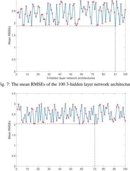
with a mean RMSE of 2.0302 (Fig. 6). The optimised 3-hidden layer network architecture is the 91st _network

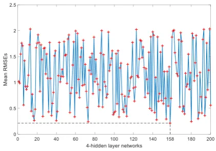
architecture with a mean RMSE of 1.8865 (Fig. 7). The optimised 4-hidden layer network architecture is the 72nd

[image:6.595.322.532.282.422.2]

network architecture with a mean RMSE of 2.0436 (Fig. 8). The 3 optimised network architectures are illustrated in Table I.

[image:6.595.310.535.450.746.2]

Fig. 6: The mean RMSEs of the 100 2-hidden layer network architectures

Fig. 7: The mean RMSEs of the 100 3-hidden layer network architectures

TABLE I: The optimised network architectures

B. Optimizing the Weights of the Optimised Network Architectures by Iterative Training and Testing (Stage 2)

The optimised 2-layer network was trained and tested iteratively 200 times on the transient dataset to further improve its performance. The mean RMSEs of the 200 networks are compared in Fig. 9. The mean RMSE of the 130th

network is the smallest (0.3434) which is much smaller than that of the optimised 2-layer network (mean RMSE of 2.0302). The optimised 3-layer network was trained and tested iteratively 200 times on the transient dataset to further improve its performance. The mean RMSEs of the 200 networks are compared in Fig. 10. The mean RMSE of the 96th network is the smallest (0.2098) which is much smaller than that of the optimised 3-layer network (mean RMSE of 1.8865). The optimised 4-layer network was trained and tested iteratively 200 times on the transient dataset to further improve its performance. The mean RMSEs of the 200 networks are compared in Fig. 11. The mean RMSE of the 158th _{network is the smallest (0.2124) which is much smaller}

[image:7.595.321.532.61.208.2]

than that of the optimised 4-layer network (mean RMSE of 2.0436).

Fig. 9: The mean RMSEs of the 200 2-hidden layer networks during iterative training-testing process.

Fig. 10: The mean RMSEs of the 200 3-hidden layer networks

Fig. 11: The mean RMSEs of the 200 4-hidden layer networks during iterative training-testing process.

C. Evaluating the Performance of the Neural Network Ensemble (Stage 3)

After the iterative training-testing process, outputs of the optimised 2-hidden layer network, the optimised 3-hidden layer network and the optimised 4-hidden layer network were combined into a NNE. The performance of the NNE was evaluated on a 25% subset of the transient dataset. The mean RMSE of the NNE is 0.1904. The RMSE of the NNE in detecting each break size is illustrated in Tables II and III. Therefore, the NNE has a better performance than the individual optimised neural networks in detecting break sizes (Table IV).

TABLE II:The RMSE OF THE NNE IN DETECTING BREAK SIZES

TABLEIII:THE RMSE OF THE NNE IN DETECTING BREAK SIZES

TABLEIV: PERFORMANCE COMPARISON

V. DISCUSSION

The good performance of the proposed constraint-based random search algorithm is due to the following key aspects of the algorithm:

1.

A good diversity of neural network architectures of high performance are created using constraint satisfaction.

2.

Optimised 2-hidden layer, 3-hidden layer and 4-hidden layer network architectures are selected by training and testing the generated network architectures on the transient dataset and a linear

Optimised Network Architectures

Architectures (inputs, hidden layers, output)

2-hidden layer architecture 37,35,13,1

3-hidden layer architecture 37,11,39,13,1

4-hidden layer architecture 37,11,22,11,48,1

Optimised Networks Mean RMSE

2-hidden layer architecture 0.3434

3-hidden layer architecture 0.2098

4-hidden layer architecture 0.2124

NNE 0.1904

Break

Size 0% 20% 40% 50% 60%

RMSE 0.0542 0.1023 0.0878 0.2084 0.1403

Break

Size 75% 100% 120% 160% 200%

[image:7.595.63.268.395.539.2] [image:7.595.62.272.572.710.2]

interpolation dataset.

3.

The performance of the optimised neural network architectures are further improved by iterative training and testing the architectures on the transient dataset.

4.

The weighted mean approach is promising in

combining the outputs of the optimised neural networks to create a NNE.

VI. CONCLUSION

This work has proposed a constraint-based random search algorithm to optimize neural network architectures and construct a NNE for detecting LOCA of NPPs. The proposed approach has achieved a high performance in detecting LOCA of NPPs. The proposed approach is a suitable approach for regression problems of different domains. Constraint satisfaction is an effective approach to create neural network architectures of high performances based on the user’s prior knowledge about neural network architectures of high performances. Future work would be to extend the random walk heuristic to generate network architectures of higher diversity and to propose new combination strategies for constructing NNEs of higher performance.

ACKNOWLEDGMENT

The authors would like to thank The Engineering and Physical Sciences Research Council (EPSRC) for their financial support under the grant number of EP/M018717/1.

REFERENCES

[1] Na MG et al (2004) Estimation of Break Location and Size for Loss of Coolant Accidents using Neural Networks. Nuclear Engineering and Design 232:289-300

[2] Le HV (2002) Large LOCA analysis of Indian Pressurized Heavy Water Reactor – 220 MWe. Nuclear Science and Technology 1:12-17 [3] Santhosh T.V. et al (2011) A Diagnostic System for Identifying

Accident Conditions in a Nuclear Reactor. Nuclear Engineering and Design 241:177-184

[4] The RELAP5-3D Code Development Team (2014) RELAP5-3D Code Manual Volume V: User's Guidelines, INL-EXT-98-00834, Revision 4.2, Idaho National Laboratory, USA

[5] Barlett EB and Uhrig RE (1992) Nuclear power plant status diagnostics using an artificial neural network. Nuclear Technology 97:272-281 [6] Guo Z, Uhrig RE (1992) Use of artificial neural networks to analyse

nuclear power plant performance. Nuclear Technology 99:36-42 [7] Bishop CM (1995) Neural networks for pattern recognition. Oxford

university press, New York, USA

[8] Bishop CM (2006) Pattern Recognition and Machine Learning. Springer, Singapore

[9] Hazewinkel M (2001) Linear interpolation. In: Hazewinkel M (ed)

Encyclopedia of Mathematics. Springer, Netherlands

[10] Han J, Kamber M, Pei J (2011) Data Mining: Concepts and Techniques (3rd edition). Morgan Kaufmann Publishers, San Francisco, CA, USA [11] Zio E, Maio FD, Stasi M (2010) A data-driven approach for predicting failure scenarios in nuclear systems. Annals of Nuclear Energy 37(4):482–491

[12] Souza TJ, Medeiros JA, Gonçalves AC (2017) Identification model of an accidental drop of a control rod in PWR reactors using thermocouple readings and radial basis function neural networks. Annals of Nuclear Energy, 103:204-211

[13] Wei X, Wan J, Zhao F (2016) Prediction Study on PCI Failure of Reactor Fuel Based on a Radial Basis Function Neural Network. Science and Technology of Nuclear Installations 2016:1-6 [14] Maio F et al (2017) Safety margin sensitivity analysis for model

selection in nuclear power plant probabilistic safety assessment. Reliability Engineering and System Safety 162:122–138

[15] Back J et al (2017) Prediction and uncertainty analysis of power peaking factor by cascaded fuzzy neural networks. Annuals of Nuclear Energy 110:989-994

[16] Krzysztof Apt. Principles of Constraint Programming. Cambridge University Press, 2003.

[17] Rina Dechter. Constraint Processing. Morgan Kaufmann Publishers Inc., 2003.

[18] Edward Tsang. Foundations of Constraint Satisfaction. Academic Press, 1993.

[19] Soares et al. Comparison of a genetic algorithm and simulated annealing for automatic neural network ensemble development. Neurocomputing. 121 (December 2013), 498-511. [20] ECLiPSe Constraint Logic Programming website.