BESSEL RANDOM VARIABLES
SARALEES NADARAJAH AND ARJUN K. GUPTA Received 20 January 2005
The distributions of products and ratios of random variables are of interest in many areas of the sciences. In this paper, the exact distributions of the product|XY|and the ratio |X/Y|are derived whenXandY are independent Bessel function random variables. An application of the results is provided by tabulating the associated percentage points.
1. Introduction
For given random variablesXandY, the distributions of the product|XY|and the ratio |X/Y|are of interest in many areas of the sciences.
In traditional portfolio selection models, certain cases involve the product of random variables. The best examples of these are in the case of investment in a number of dif-ferent overseas markets. In portfolio diversification models (see, e.g., Grubel [6]), not only are prices of shares in local markets uncertain, but also the exchange rates are un-certain so that the value of the portfolio in domestic currency is related to a product of random variables. Similarly in models of diversified production by multinationals (see, e.g., Rugman [21]), there are local production uncertainty and exchange rate uncertainty so that profits in home currency are again related to a product of random variables. An entirely different example is drawn from the econometric literature. In making a forecast from an estimated equation, Feldstein [4] pointed out that both the parameter and the value of the exogenous variable in the forecast period could be considered as random variables. Hence, the forecast was proportional to a product of random variables.
An important example of ratios of random variables is the stress-strength model in the context of reliability. It describes the life of a component which has a random strengthY and is subjected to random stressX. The component fails at the instant that the stress applied to it exceeds the strength and the component will function satisfactorily when-everY > X. Thus, Pr(X < Y) is a measure of component reliability. It has many applica-tions especially in engineering concepts such as structures, deterioration of rocket mo-tors, static fatigue of ceramic components, fatigue failure of aircraft structures, and the aging of concrete pressure vessels.
The distributions of|XY|and|X/Y|have been studied by several authors especially whenXandY are independent random variables and come from the same family. With Copyright©2005 Hindawi Publishing Corporation
respect to products of random variables, see Sakamoto [22] for uniform family, Harter [7] and Wallgren [28] for Student’stfamily, Springer and Thompson [24] for normal family, Stuart [26] and Podolski [14] for gamma family, Steece [25], Bhargava and Khatri [3], and Tang and Gupta [27] for beta family, Abu-Salih [1] for power function family, and Malik and Trudel [11] for exponential family (see also Rathie and Rohrer [20] for a comprehensive review of known results). With respect to ratios of random variables, see Marsaglia [12] and Korhonen and Narula [9] for normal family, Press [15] for Student’st family, Basu and Lochner [2] for Weibull family, Shcolnick [23] for stable family, Hawkins and Han [8] for noncentral chi-square family, Provost [16] for gamma family, and Pham-Gia [13] for beta family.
In this paper, we study the exact distributions of|XY|and|X/Y|whenXandY are independent Bessel function random variables with pdfs
fX(x)= |x| m
√
π2mbm+1Γ(m+ 1/2)Km
xb, (1.1)
fY(y)= |y| n
√
π2nβn+1Γ(n+ 1/2)Kn
yβ, (1.2)
respectively, for−∞< x <∞,−∞< y <∞,b >0,β >0,m >1, andn >1, where
Kν(x)= √
πxν 2νΓ(ν+ 1/2)
∞
1
t2−1ν−1/2exp(−xt)dt (1.3)
is the modified Bessel function of the third kind. Tabulations of the associated percentage points are also provided.
Bessel function distributions have found applications in a variety of areas that range from image and speech recognition and ocean engineering to finance. They are rapidly becoming distributions of first choice whenever “something” heavier than Gaussian tails is observed in the data. Some examples are as follows (see Kotz et al. [10] for further applications).
(1) In communication theory,X andY could represent the random noises corre-sponding to two different signals.
(2) In ocean engineering,XandYcould represent distributions of navigation errors. (3) In finance,XandY could represent distributions of log-returns of two different
commodities.
The exact expressions for the distributions of the product and ratio are given in Sec-tions2and3of the paper. The calculations involve the generalized hypergeometric func-tion defined by
pFq
a1,...,ap;b1,...,bq;x
=∞
k=0
a1ka2k···ap
k
b1kb2k···bq
k
xk
k!, (1.4)
where (e)k=e(e+ 1)···(e+k−1) denotes the ascending factorial. We also need the following important lemmas.
Lemma 1.1 (Prudnikov et al. [18, equation (2.16.33.5), Volume 2]). For b >0 and c >0,
∞
0 x
α−1K
µ
b x
Kν(cx)dx
=2α−2µ−3bµcµ−αΓ(−µ)Γα+ν−µ
2
Γα−ν−µ 2
×0F3
1 +µ, 1 +µ−ν−α 2 , 1 +
ν+µ−α
2 ;
b2c2 16
+ 2α+2µ−3b−µc−µ−αΓ(µ)Γα+ν+µ
2
Γα−ν+µ 2
×0F3
1−µ, 1−α+µ+ν 2 , 1−
α+µ−ν
2 ;
b2c2 16
+ 2−α−2ν−3bα+νcνΓ(−ν)Γµ−ν−α
2
Γ−µ+ν+α 2
×0F3
1 +ν, 1 +α+ν−µ 2 , 1 +
α+µ+ν
2 ;
b2c2 16
+ 22ν−α−3bα−νc−νΓ(ν)Γµ+ν−α 2
Γν−µ2−α
×0F3
1−ν, 1 +α−µ−ν 2 , 1 +
α+µ−ν
2 ;
b2c2 16
.
(1.5)
Lemma1.2 (Gradshteyn and Ryzhik [5, equation (6.576.4)]). Fora+b >0andλ <1− µ−ν,
∞
0 x −λK
µ(ax)Kν(bx)dx=2
−2−λa−ν+λ−1bν
Γ(1−λ) Γ 1−
λ+µ+ν 2
Γ1−λ−2µ+ν
×Γ1−λ+2µ−νΓ1−λ−2µ−ν
×2F1 1−
λ+µ+ν
2 ,
1−λ−µ+ν
2 ; 1−λ; 1− b2 a2
.
Lemma 1.3 (Prudnikov et al. [19, equation (2.21.1.14), Volume 3]). For y >0,β >0, α+β <1 +a, andα+β <1 +b,
∞
y x α−1(
x−y)β−12F1(a,b;c; 1−wx)dx
=w−ayα+β−a−1Γ(c)Γ(b−a)Γ(β)Γ(a−α−β+ 1)
Γ(b)Γ(c−a)Γ(a−α+ 1) ×3F2
a,c−b,a−α−β+ 1;a−α+ 1,a−b+ 1; 1 wy
+w−byα+β−b−1Γ(c)Γ(a−b)Γ(β)Γ(b−α−β+ 1)
Γ(a)Γ(c−b)Γ(b−α+ 1) ×3F2
b,c−a,b−α−β+ 1;b−a+ 1,b−α+ 1; 1 wy
.
(1.7)
Lemma 1.4 (Prudnikov et al. [19, equation (2.22.2.1), Volume 3]). For a >0, α >0, β >0, andp≤q+ 1,
a
0x
α−1(a−x)β−1
pFqa1,...,ap;b1,...,bq;wxdx
=aα+β−1B(α,β)
p+1Fq+1
a1,...,ap,α;b1,...,bq,α+β;aw.
(1.8)
Further properties of the generalized hypergeometric function can be found in Prud-nikov et al. [17,18,19] and Gradshteyn and Ryzhik [5].
2. Product
Theorem 2.1derives explicit expressions for the distribution of|XY|in terms of the0F3 and1F4hypergeometric functions.
Theorem2.1. Suppose thatX andY are distributed according to (1.1) and (1.2), respec-tively. The pdf and the cdf ofZ= |XY|can be expressed as
fZ(z)=K2n−3m−1b−mβn−2mΓ2(−m)Γ(n−m)z2mC1(z)−2m+nbmβnCΓ(m)Γ(n)C2(z)
+ 2m−3n−1bm−2nβ−nΓ2(−n)Γ(m−n)z2nC3(z) ,
(2.1) FZ(z)=K
2n−3m−1b−mβn−2mΓ2(−m)Γ(n−m)z2m+1
2m+ 1C4(z)−2m
+nbmβnCΓ(m)Γ(n)zC5(z)
+ 2m−3n−1bm−2nβ−nΓ2(−n)Γ(m−n)z 2n+1
2n+ 1C6(z)
,
where
C1(z)=0F3
1 +m, 1 +m−n, 1 +m; z 2
16b2β2
,
C2(z)=0F3
1−m, 1−n, 1; z 2
16b2β2
,
C3(z)=0F3
1 +n, 1 +n−m, 1 +n; z 2
16b2β2
,
C4(z)=1F4 1
2+m; 1 +m, 1 +m−n, 1 +m, 3 2+m;
z2 16b2β2
,
C5(z)=1F4 1
2; 1−m, 1−n, 1, 3 2;
z2 16b2β2
,
C6(z)=1F4 1
2+n; 1 +n, 1 +n−m, 1 +n, 3 2+n;
z2 16b2β2
, 1
K =π2m
+nbm+1βn+1Γm+1 2
Γn+1 2
,
(2.3)
andCdenotes Euler’s constant.
Proof. The pdf of|XY|can be expressed as
fZ(z)=4
∞
0 1 yfX
z y
fY(y)dy
=4 ∞ 0 1 y |z/y|m √
π2mbm+1Γ(m+ 1/2)Km
byz √ |y|n
π2nβn+1Γ(n+ 1/2)Kn
βydy
= zmI(m,n)
π2m+n−2bm+1βn+1Γ(m+ 1/2)Γ(n+ 1/2),
(2.4) whereI(m,n) denotes the integral
I(m,n)= ∞
0 y
n−m−1 Km z by Kn y β dy. (2.5)
The result in (2.1) follows by direct application ofLemma 1.1to calculateI(m,n). The cdf ofZcan be expressed as
FZ(z)=K
2n−3m−1b−mβn−2mΓ2(−m)Γ(n−m) z
0w
2mC1(w)dw
−2m+nbmβnCΓ(m)Γ(n) z
0C2(w)dw + 2m−3n−1bm−2nβ−nΓ2(−n)Γ(m−n)
z
0w
2nC3(w)dw.
(2.6)
0 1 2 3 4 5
z n=2
n=3 nn==510 0
0.1
0.2
(a)
0 1 2 3 4 5
z n=2
n=3 nn==510 0
0.1
0.2
(b)
0 1 2 3 4 5
z
n=2
n=3 nn==510 0
0.1
0.2
(c)
0 1 2 3 4 5
z
n=2
n=3 nn==510 0
0.1
0.2
[image:6.468.57.411.75.483.2](d)
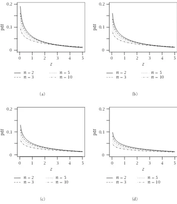
Figure 2.1. Plots of the pdf (2.1) forb=1,β=1, and (a)m=2; (b)m=3; (c)m=5; and (d)m=10.
Figure 2.1illustrates possible shapes of the pdf (2.1) for selected values ofmandn. The four curves in each plot correspond to selected values ofn. The effect of the parameters is evident.
3. Ratio
Theorem3.1. Suppose thatX andY are distributed according to (1.1) and (1.2), respec-tively. The pdf and the cdf ofZ= |X/Y|can be expressed as
fZ(z)=2L(β/b)
−2n−1
m+n+ 1 z
−2n−2D1(z), (3.1)
FZ(z)=2LΓ(m+n+ 1)
Γ(−m) D2(z) (2m+ 1)Γ(n+ 1)+
βzD3(z) mbΓ(m+n+ 1)
, (3.2)
where
D1(z)=2F1
m+n+ 1,n+ 1;m+n+ 2; 1− b2 β2z2
,
D2(z)=2F1
m+n+ 1,m+1 2;m+
3 2;
β2z2 b2
,
D3(z)=3F2
n+ 1, 1,1 2; 1−m,
3 2;
β2z2 b2
,
L= Γ(m+ 1)Γ(n+ 1) πΓ(m+ 1/2)Γ(n+ 1/2).
(3.3)
Proof. The pdf ofZ= |X/Y|can be expressed as
fZ(z)=4
∞
0 y fX(yz)fY(y)dy =4
∞
0 y
(yz)m
√
π2mΓ(m+ 1/2)Km(yz)
yn
√
π2nΓ(n+ 1/2)Kn(y)dy
= zmI(m,n)
π2m+n−2Γ(m+ 1/2)Γ(n+ 1/2),
(3.4)
whereI(m,n) denotes the integral
I(m,n)= ∞
0 y
m+n+1
Km(yz)Kn(y)dy. (3.5)
The result in (3.1) follows by direct application ofLemma 1.2to calculateI(m,n). The cdf ofZcan be expressed as
FZ(z)=
2L(β/b)−2n−1 m+n+ 1
z
0w
−2n−2D1(w)dw
= L
m+n+ 1 ∞
b2/(βz)2x n−1/2
2 F1(m+n+ 1,n+ 1;m+n+ 2; 1−x)dx,
(3.6)
which follows by settingx=(βw/b)−2. The result in (3.2) follows by applyingLemma 1.3
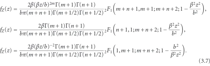
Using special properties of the 2F1 hypergeometric function, one can derive other equivalent forms and elementary forms for the pdf ofZ= |X/Y|. This is illustrated in the corollaries below.
Corollary3.2. The pdf given by (3.1) can be expressed in the equivalent forms
fZ(z)= 2β(βz/b)
2mΓ(m+ 1)Γ(n+ 1)
bπ(m+n+ 1)Γ(m+ 1/2)Γ(n+ 1/2)2F1
m+n+ 1,m+ 1;m+n+ 2; 1−β2z2 b2
,
fZ(z)=bπ(m+2nβ+ 1)Γ(mΓ+ 1)(m+ 1Γ(n/2)+ 1)Γ(n+ 1/2)2F1
n+ 1, 1;m+n+ 2; 1−β2z2 b2
,
fZ(z)=
2β(βz/b)−2Γ(m+ 1)Γ(n+ 1) bπ(m+n+ 1)Γ(m+ 1/2)Γ(n+ 1/2)2F1
1,m+ 1;m+n+ 2; 1− b2 β2z2
.
(3.7)
Corollary3.3. Ifm≥2andn≥2are integers, then (3.1) can be reduced to the elementary form
fZ(z)= 2βΓ(m+ 1)Γ(m+n+ 1)
bπβ2z2/b2−1Γ(m+ 1/2)Γ(n+ 1/2)
× n
k=1
(n−k)!1−β2z2/b21−k (m+n+ 1−k)! +
1−β2z2/b21−n m!β2z2/b2
×
−2
1− b2 β2z2
−m−1 log
βz
b
+
m
k=1
1−b2/β2z2−k m+ 1−k
.
(3.8)
Corollary3.4. Ifm−1/2≥1andn−1/2≥1are integers, then (3.1) can be reduced to the elementary form
fZ(z)= 2b
1−β2z2/b2−m−n−1Γ(m+ 1)Γ(n+ 1) βz2π(m+n+ 1)(−m−1)
m+n+2Γ(m+ 1/2)Γ(n+ 1/2)
×
Γ(−m) βz
b 2m+2
+
m+n+1
k=1
(−m−1)k(−1)k
1− b2
β2z2 k−1
(βz/b)2k
. (3.9)
[image:8.468.63.413.138.249.2]4. Percentiles
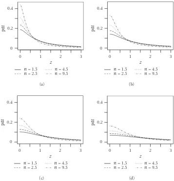
Figure 4.1illustrates possible shapes of the pdf (3.1) for selected values ofmandn. The four curves in each plot correspond to selected values ofn. The effect of the parameters is evident.
0 1 2 3
z n=1.5
n=2.5 nn==49..55 0
0.2
0.4
(a)
0 1 2 3
z n=1.5
n=2.5 nn==49..55 0
0.2
0.4
(b)
0 1 2 3
z n=1.5
n=2.5 nn==49..55 0
0.2
0.4
(c)
0 1 2 3
z n=1.5
n=2.5 nn==49..55 0
0.2
0.4
[image:9.468.56.413.76.448.2](d)
Figure 4.1. Plots of the pdf (3.1) forb=1,β=1, and (a)m=1.5; (b)m=2.5; (c)m=4.5; and (d) m=9.5.
the equations
K
2n−3m−1b−mβn−2mΓ2(−m)Γ(n−m) z 2m+1
p
2m+ 1C4
zp
−2m+nbmβnCΓ(m)Γ(n)z pC5
zp
+ 2m−3n−1bm−2nβ−nΓ2(−n)Γ(m−n)z 2n+1
p
2n+ 1C6
zp
=p,
2LΓ(m+n+ 1)
Γ(−m)D2z
p
(2m+ 1)Γ(n+ 1)+
βzpD3
zp
mbΓ(m+n+ 1)
=p.
Table 4.1. Percentage pointszpofZ= |XY|.
m n p=0.6 p=0.7 p=0.8 p=0.9 p=0.95 p=0.99 2 2 0.02903867 0.0609406 0.1328627 0.3470357 0.6927036 2.098452 2 3 0.07362923 0.1376486 0.2682605 0.6146536 1.130666 3.038813 2 4 0.1100132 0.1998708 0.3777723 0.827011 1.465626 3.755526 2 5 0.1408100 0.2514674 0.4678341 1.000369 1.752475 4.380899 2 6 0.1673438 0.2968515 0.5449642 1.151051 1.991074 4.848271 2 7 0.1906657 0.3359331 0.6139745 1.284624 2.218128 5.323573 2 8 0.2125461 0.372798 0.6770319 1.415690 2.416419 5.745124 2 9 0.2300810 0.4031021 0.7305227 1.517905 2.591786 6.145533 3 3 0.1744381 0.2938927 0.5183827 1.057357 1.798354 4.335123 3 4 0.2572388 0.4184127 0.711219 1.388183 2.282625 5.225012 3 5 0.3263338 0.5227913 0.870987 1.660568 2.691937 6.044048 3 6 0.3860577 0.6124857 1.011584 1.908407 3.049341 6.677126 3 7 0.4394194 0.6929521 1.137077 2.125184 3.382392 7.385786 3 8 0.4865918 0.7648362 1.249936 2.318062 3.661295 7.867155 3 9 0.5306344 0.8335735 1.356932 2.498872 3.923604 8.372842 4 4 0.3773593 0.593275 0.972541 1.816783 2.900670 6.372728 4 5 0.4760256 0.7359029 1.184584 2.162823 3.404096 7.3069 4 6 0.5626443 0.8623236 1.371957 2.474747 3.845828 8.08524 4 7 0.638364 0.9744115 1.541777 2.752022 4.246468 8.858037 4 8 0.7085111 1.076598 1.696747 3.004645 4.632417 9.46566 4 9 0.7702856 1.166607 1.830414 3.240364 4.958135 10.19733 5 5 0.6033154 0.9178398 1.450584 2.584631 3.999764 8.318145 5 6 0.7075169 1.066605 1.668016 2.942446 4.50238 9.176312 5 7 0.8076738 1.211170 1.883969 3.282990 4.993118 10.06218
5 8 0.89244 1.334572 2.062933 3.568706 5.40753 10.82776
5 9 0.974915 1.449774 2.230274 3.847315 5.804434 11.49615 6 6 0.8362517 1.250325 1.934166 3.357292 5.101803 10.24216 6 7 0.9532409 1.417497 2.175916 3.744367 5.625393 11.18685
6 8 1.053948 1.559225 2.37994 4.067588 6.09969 11.93585
6 9 1.151888 1.695543 2.583201 4.397424 6.553556 12.80644 7 7 1.083447 1.595423 2.431431 4.140509 6.192786 12.20569 7 8 1.198694 1.763451 2.676427 4.537504 6.72858 13.04854 7 9 1.308068 1.918944 2.897775 4.865201 7.179527 13.83574 8 8 1.331007 1.948211 2.941492 4.955321 7.298417 14.03725 8 9 1.450212 2.113748 3.176776 5.310468 7.810788 14.88969 9 9 1.588348 2.305376 3.451306 5.742988 8.420277 15.94564
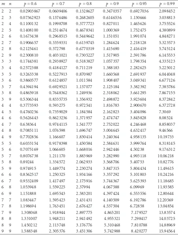
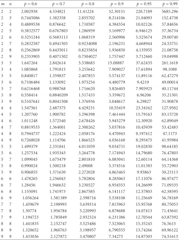
Evidently, this involves computation of the generalized hypergeometric function and rou-tines for this are widely available. We used the function hypergeom (·) in the algebraic manipulation package Maple. Tables4.1and4.2provide the numerical values ofzp for
Table 4.2. Percentage pointszpofZ= |X/Y|.
m n p=0.6 p=0.7 p=0.8 p=0.9 p=0.95 p=0.99 2 2 2.002938 4.334821 11.41224 52.30151 220.7189 5685.296 2 3 0.7445086 1.382358 2.855702 8.214106 21.04093 152.4738 2 4 0.4889538 0.876642 1.710587 4.384554 10.02126 57.84656 2 5 0.3832577 0.6767803 1.286959 3.169977 6.946125 37.36734 2 6 0.3251244 0.5683113 1.068319 2.560906 5.525674 29.00740 2 7 0.2832587 0.4941505 0.9234088 2.196231 4.668944 24.53751 2 8 0.2562869 0.4435011 0.8235854 1.936850 4.135955 21.08758 2 9 0.2353905 0.4071502 0.7504027 1.757447 3.712460 19.04998 3 3 1.647264 2.842614 5.538683 15.08887 37.62435 261.1618
3 4 1.085868 1.791815 3.255642 7.909027 17.61894 98.1088
3 5 0.840817 1.359837 2.407853 5.574137 11.89116 62.47279
3 6 0.7106484 1.133092 1.975254 4.480779 9.4219 49.00014
3 7 0.6216468 0.988768 1.716620 3.826405 7.905925 40.11744 3 8 0.558414 0.8840209 1.517433 3.359672 6.96206 35.21301 3 9 0.5107641 0.8041508 1.376936 3.048617 6.29827 31.90878 4 4 1.547561 2.487375 4.429231 10.55419 23.34162 127.9502 4 5 1.207760 1.900782 3.296398 7.461444 15.79163 83.15728 4 6 1.011248 1.572540 2.678426 5.945279 12.30920 62.89049 4 7 0.8819533 1.364001 2.300262 5.037816 10.45939 53.42483 4 8 0.7944737 1.222424 2.058176 4.470943 9.197412 47.1173 4 9 0.7268028 1.114706 1.866525 4.036168 8.295475 41.95984 5 5 1.499379 2.331841 4.011059 9.034731 19.02830 98.64185 5 6 1.257534 1.935343 3.264778 7.174943 14.79680 76.47803 5 7 1.099045 1.675479 2.801810 6.083041 12.60114 64.14368
5 8 0.990024 1.500218 2.49008 5.374516 11.01383 55.72903
5 9 0.906855 1.371630 2.272028 4.863465 9.93863 50.23113
6 6 1.478265 2.256043 3.782804 8.285063 17.11076 86.97477
6 7 1.28456 1.946632 3.230527 6.954553 14.26699 71.09335
6 8 1.155091 1.741973 2.867585 6.141117 12.57803 62.58595 6 9 1.056264 1.581389 2.598716 5.538108 11.25649 56.78169 7 7 1.459679 2.198993 3.639314 7.815963 15.95768 80.75053
7 8 1.30774 1.956784 3.220993 6.878688 14.07413 71.43641
7 9 1.194723 1.785849 2.932324 6.231386 12.70544 63.87592 8 8 1.441835 2.152747 3.525486 7.523065 15.35245 76.5615 8 9 1.320652 1.960763 3.198957 6.790555 13.74266 69.96122
9 9 1.433036 2.127872 3.470807 7.34273 14.87503 74.51613
Besides being of practical interest, the above tables can be used to check the accuracy of the results derived in Sections2and3. We estimated the relevant percentage points by simulating samples of size 108from the two Bessel function distributions. The estimates were consistent with the tabulated values up to the third decimal place.
Acknowledgment
The authors would like to thank the referee and the Associate Editor for carefully reading the paper and for their help in improving the paper.
References
[1] M. S. Abu-Salih,Distributions of the product and the quotient of power-function random vari-ables, Arab J. Math.4(1983), no. 1-2, 77–90.
[2] A. P. Basu and R. H. Lochner,On the distribution of the ratio of two random variables having generalized life distributions, Technometrics13(1971), 281–287.
[3] R. P. Bhargava and C. G. Khatri,The distribution of product of independent beta random variables with application to multivariate analysis, Ann. Inst. Statist. Math.33(1981), no. 2, 287–296. [4] M. S. Feldstein,The error of forecast in econometric models when the forecast-period exogenous
variables are stochastic, Econometrica39(1971), 55–60.
[5] I. S. Gradshteyn and I. M. Ryzhik,Table of Integrals, Series, and Products, 6th ed., Academic Press, California, 2000.
[6] H. G. Grubel,Internationally diversified portfolios: welfare gains capital flows, American Eco-nomic Review58(1968), 1299–1314.
[7] H. L. Harter,On the distribution of Wald’s classification statistic, Ann. Math. Statistics22(1951), 58–67.
[8] D. L. Hawkins and C.-P. Han,Bivariate distributions of some ratios of independent noncentral chi-square random variables, Comm. Statist. A—Theory Methods15(1986), no. 1, 261– 277.
[9] P. J. Korhonen and S. C. Narula,The probability distribution of the ratio of the absolute values of two normal variables, J. Statist. Comput. Simulation33(1989), no. 3, 173–182.
[10] S. Kotz, T. J. Kozubowski, and K. Podg ´orski,The Laplace Distribution and Generalizations. A Re-visit with Applications to Communications, Economics, Engineering, and Finance, Birkh¨auser Boston, Massachusetts, 2001.
[11] H. J. Malik and R. Trudel,Probability density function of the product and quotient of two corre-lated exponential random variables, Canad. Math. Bull.29(1986), no. 4, 413–418.
[12] G. Marsaglia,Ratios of normal variables and ratios of sums of uniform variables, J. Amer. Statist. Assoc.60(1965), 193–204.
[13] T. Pham-Gia,Distributions of the ratios of independent beta variables and applications, Comm. Statist. Theory Methods29(2000), no. 12, 2693–2715.
[14] H. Podolski,The distribution of a product ofnindependent random variables with generalized gamma distribution, Demonstratio Math.4(1972), 119–123.
[15] S. J. Press,Thet-ratio distribution, J. Amer. Statist. Assoc.64(1969), 242–252.
[16] S. B. Provost,On the distribution of the ratio of powers of sums of gamma random variables, Pakistan J. Statist.5(1989), no. 2, 157–174.
[17] A. P. Prudnikov, Y. A. Brychkov, and O. I. Marichev,Integrals and Series. Vol. 1: Elementary Functions, Gordon & Breach Science, New York, 1986.
[19] ,Integrals and Series. Vol. 3: More Special Functions, Gordon & Breach Science, New York, 1990.
[20] P. N. Rathie and H. G. Rohrer,The exact distribution of products of independent random vari-ables, Metron45(1987), no. 3-4, 235–245.
[21] A. M. Rugman,International Diversification and the Multinational Enterprise, Lexington, Mas-sachusetts, 1979.
[22] H. Sakamoto,On the distributions of the product and the quotient of the independent and uni-formly distributed random variables, T ˆohoku Math. J.49(1943), 243–260.
[23] S. M. Shcolnick,On the ratio of independent stable random variables, Stability Problems for Stochastic Models (Uzhgorod, 1984), Lecture Notes in Math., vol. 1155, Springer, Berlin, 1985, pp. 349–354.
[24] M. D. Springer and W. E. Thompson,The distribution of products of beta, gamma and Gaussian random variables, SIAM J. Appl. Math.18(1970), 721–737.
[25] B. M. Steece,On the exact distribution for the product of two independent beta-distributed ran-dom variables, Metron34(1976), no. 1-2, 187–190 (1978).
[26] A. Stuart,Gamma-distributed products of independent random variables, Biometrika49(1962), 564–565.
[27] J. Tang and A. K. Gupta,On the distribution of the product of independent beta random variables, Statist. Probab. Lett.2(1984), no. 3, 165–168.
[28] C. M. Wallgren,The distribution of the product of two correlatedtvariates, J. Amer. Statist. Assoc. 75(1980), no. 372, 996–1000.
Saralees Nadarajah: Department of Statistics, College of Arts and Sciences, University of Nebraska, Lincoln, NE 68583-0712, USA
E-mail address:[email protected]
Arjun K. Gupta: Department of Mathematics and Statistics, College of Arts and Sciences, Bowling Green State University, Bowling Green, OH 43403-0221, USA