GE-INTERNATIONAL JOURNAL OF ENGINEERING RESEARCH
VOLUME -2, ISSUE -4 (JUNE 2014) ISSN: (2321-1717)
A HEURISTIC ALGORITHM TO SOLVE TSP FOR A PARTICULAR TYPE OF
HAMILTONIAN GRAPH
Kanak Chandra Bora,
Computer Science & Engineering, Research Scholar, Gauhati University,
Jalukbari, Assam, India.
Bichitra Kalita,
Master of Computer Application, Assam Engineering College,
Jalukbari, Assam, India.
ABSTRACT
A heuristic algorithm has been developed to find out the least cost route (minimum weighted
Hamiltonian circuit) for a particular type of weighted graph G (3m + 7, 6m + 16) for m ≥ 1, which is
planar, non-regular, non-bipartite and Hamiltonian related with traveling salesman problem.
KEYWORDS- HAMILTONIAN CIRCUIT, HEURISTIC ALGORITHM, NON-REGULAR,
TRAVELING SALESMAN PROBLEM.
1. Introduction
The Traveling Salesman Problem(TSP) is a well known NP-complete problem [1-2]. TSP is used to
model several real world industrial problems [3]. There are some exact approaches for TSP like
Lagragean relaxation [4] and branch and bound [5] which are successfully used relatively for small
size problems. In an n-city TSP problem permutation of n will give the solution and hence for larger
size of problem exact algorithm is not suitable. Therefore many heuristic algorithms have been
developed to solve the traveling salesman problem like - Ant Colony Optimization [6], Greedy
Algorithm [8], Bee Colony Optimization [3], Firefly Algorithm [7], Hybrid Metaheuristics
Algorithm,[9], Genetic Algorithm [10]. These algorithms are generally for complete graph.
Here one particular type of weighted graph G (3m + 7, 6m + 16) for m ≥1, which is planar,
non-regular, non-bipartite and Hamiltonian is considered from [11] for the application of traveling
salesman problem. It has been reported that many heuristic algorithms have been established for
complete and non complete graphs. Various properties of Hamiltonian sub-graph of the complete
graph K2m + 3 for m ≥ 2 have been studied and an algorithm has also been developed for the traveling salesman problem by Kalita, B [12] for different values of m ≥2 . Another algorithm has also been
GE-INTERNATIONAL JOURNAL OF ENGINEERING RESEARCH
VOLUME -2, ISSUE -4 (JUNE 2014) ISSN: (2321-1717)
sub-graph of the complete graph K2m + 2 was studied by Dutta, Anupam et al [14] and an algorithm was also developed for the solution of traveling salesman problem. Choudhury Jayanta Kr. et al discussed
the different type of factorization of graphs of the complete graphs K6m + 2 ,K6m – 2, and K6m for m ≥ 1 and developed an algorithm different from the above algorithms for the solution of traveling salesman
problem [15]. Recently, Choudhury, Jayanta Kr. et al discussed the decomposition of complete graphs
K2m + 1 for m ≥ 2 into circulant graphs with various properties. In addition to this, an algorithm has also been discussed for traveling salesman problem under different situations for the said graphs [16].
Besides, Choudhury, Jayanta Kr. and Kalita, B., discussed the generation of a maximal triangle free
graph from the complete graph K2m +3 , for m ≥ 2 and an algorithm was also developed under different cases to solve the traveling salesman problem of the complete graph K2m + 3 [17]. Since the traveling salesman problems is an NP-complete problems, and there is no polynomial time algorithm, hence
there is need to study it for various types of weighted graph. Here, a complete, bipartite,
non-regular but Hamiltonian graph of particular type has been considered.
This paper is organized in three sections. In section 1, introduction is given. In section-2,
construction of the particular type of graphs is discussed. In section 3, an algorithm is developed and
in section 4, experimental result is cited.
2. Construction of the Particular Type of Graphs
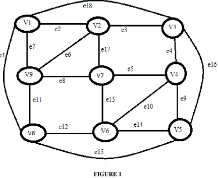
Let us consider the graph G(3m + 6, 12 + 6m) for m ≥ 1, which is regular of degree four,
non-bipartite and planner having two edge-disjoint Hamiltonian cycles and two equal path partitions as
GE-INTERNATIONAL JOURNAL OF ENGINEERING RESEARCH
VOLUME -2, ISSUE -4 (JUNE 2014) ISSN: (2321-1717)
FIGURE 1
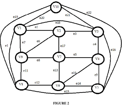
Now adding one vertex outer side the region of the graph for m=1 in such a way that the
degree of the added vertex is four [Figure-2]. Continuing the process of construction for different values of m =2,3,4,5,………keeping in mind for added vertex is of degree four and the graph
thus obtained is of the G(3m + 7, 16 + 6m) for m ≥ 1, which is planar, non-regular, non-bipartite but
GE-INTERNATIONAL JOURNAL OF ENGINEERING RESEARCH
VOLUME -2, ISSUE -4 (JUNE 2014) ISSN: (2321-1717)
FIGURE 2
Now making this graph as weighted graph introducing the weight to the edges of this graph an
algorithm has been developed in section 3.
3. Algorithm
Here an algorithm has been developed to find the minimum cost route of a particular type of weighted graph G (3m + 7, 6m + 16) for m ≥1, which is planar, non-regular, non-bipartite and Hamiltonian.
The following steps are considered.
Step 1: Find the total weight of each vertex adding the weight of edges incident to that vertex of the
graph G (3m + 7, 6m + 16) from the cost matrix.
Step 2: Arrange the vertices in descending order as per total weight of each vertex, as stated in step-1.
Step 3: Consider one by one all the vertices obtained in the descending order one after another and
select the edges of smallest weighted incident with those vertices and these edges are kept in
GE-INTERNATIONAL JOURNAL OF ENGINEERING RESEARCH
VOLUME -2, ISSUE -4 (JUNE 2014) ISSN: (2321-1717)
Step 4: Connect the selected edges from the array serially in the same order as they were kept. If there
are more than two edges from a particular vertex are selected then the first two edges only will
be connected from the array and the remaining edges will be discarded.
Step 5: Study the sub-graph obtained after connection of edges as stated in step 4. If the sub graph is
connected then go to step-6 otherwise go to step-8.
Step 6: Check for one degree vertices. If there are one degree vertices then connect them and then the
required least cost route Hamiltonian circuit is obtained .Then go to step-14.
Step 7: If there are no one degree vertices of the sub graph obtained from step 4, then go to step 14.
Step 8: Study the components of the sub graph obtained in step-4. If there is isolated vertex then go to
step-9 otherwise go to step-11.
Step 9: For each isolated vertex, lower to higher weighted edges one after another is considered to get
connection. Three cases arise here.
Case-(a): Isolated vertex is connected to a one degree vertex. If there is no more isolated vertex, then
go to step-10, otherwise step-9 is repeated for the isolated vertex again.
Case-(b): Isolated vertex is connected to a vertex whose degree becomes 3 and the weight of the
newly connected edge is less than the previously connected edges. Then the higher weighted
edge from the connected vertex already considered at step -4, gets deleted. If there is no
isolated vertex, then go to step-10, otherwise step-9 is repeated for the isolated vertex
again.
Case-(c): Isolated vertex is connected to a vertex whose degree becomes 3 and the weight of the
newly connected edge is greater than the weight of the existing edges. Then the newly
connected edge is discarded and then the next least cost edge is considered for connection.
Step- 10: Examine the one degree vertices in the sub graph. If there is lesser weighted edge from any
one degree vertices to other vertex and connecting this edge, degree of any vertex
becomes 3 then the highest weighted edge of the existing two edges gets deleted. If any
vertex becomes isolate, then go to step 9, otherwise go to step -11.
Step-11: Check for one possible edge for the vertices of one degree in the same order as obtained at
step-2. (One possible edge means from a particular vertex there is only one edge ,
connection of which will not create any cycle of length less than n, the number of vertices of
the graph and degree of any vertex will not be greater than 2.). If there are two one possible
GE-INTERNATIONAL JOURNAL OF ENGINEERING RESEARCH
VOLUME -2, ISSUE -4 (JUNE 2014) ISSN: (2321-1717)
lesser weighted edge will be connected. If there is one possible edge then it is connected
and after this if any new one possible edge generated then it is connected repeatedly. If one
degree vertices are remain then go to step-12, otherwise go to step-14.
Step-12: If there is connectivity problem then go to step-13, otherwise highest weighted one degree
vertex is connected with the next possible least cost edge. If any one possible edge is
generated then go to step-11, otherwise step-12 is repeated. (Connectivity problem means
there are two one degree vertices in the sub graph and there is no possible edge connection
between the two one degree vertices).
Step-13: There are two cases.
Case-(a): Lesser weighted edge is available from one degree vertex.
Case-(i) From both the one degree vertices have lesser weighted edge to other 2 degree vertex. If both
the vertices have equal total weight as obtained at step-1, then one degree vertex is
connected with lesser weighted edge arbitrarily which will not create any circuit of length less
than n (where n is the total number of vertices in the graph) and due to this edge connection,
higher weighted edge is deleted from the connected vertex to make the degree of the vertex 2.
If both the vertices do not have equal total weight then highest weight one degree vertex is
considered for connection if it does not create cycle of length lesser than length n,
otherwise next one degree vertex is considered for connection.. This considered vertex is
connected with the next lesser weighted possible edge and due to this connection one
higher weighted edge is deleted from the degree three vertex. If isolated vertex is generated
then go to step-9, otherwise go to step-11.
Case-(ii) Only from one of the two one degree vertices has lesser weighted edge. Lesser weighted
edge is connected and one higher weighted edge is deleted to make degree of the vertex 2 or
another edge is deleted to break the cycle of length lesser than n. If any isolated vertex is
generated then go to step-9, otherwise go to step-11.
Case-(b): Lesser weighted edge is not available from one degree vertex to other vertex. Highest
weight one degree vertex is connected with the next lesser weighted edge and the degree of
the connected vertex has become 3 and a cycle of length less than n (where n is the
number of vertices of the given graph) is also formed. And then particular edge from the
degree 3 vertex gets deleted to break the cycle. And then go to step-11.
GE-INTERNATIONAL JOURNAL OF ENGINEERING RESEARCH
VOLUME -2, ISSUE -4 (JUNE 2014) ISSN: (2321-1717)
Note: At step-13, once an edge is deleted that cannot be connected again.
4. Experimental Results
The different cases for the experimental results [1-3] have been cited.
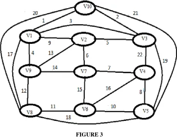
Experimental Result: [1]. Let us consider the graph of Figure 3 for m=1.
FIGURE 3
[image:7.595.121.485.190.473.2]The cost matrix of the graph and as per step-1, total weight of each vertex is calculated in table 1.
TABLE 1
V1 V2 V3 V4 V5 V6 V7 V8 V9 V10 Total weight
V1 9 3 17 4 1 34
V2 9 5 6 13 33
V3 3 5 22 19 2 51
V4 22 8 16 7 53
V5 19 8 10 18 21 76
GE-INTERNATIONAL JOURNAL OF ENGINEERING RESEARCH
VOLUME -2, ISSUE -4 (JUNE 2014) ISSN: (2321-1717)
V7 6 7 15 14 42
V8 17 18 11 12 20 78
V9 4 13 14 12 43
V10 1 2 21 20 44
As per step-2, vertices are arranged in descending orders are V8, V5, V4, V6, V3, V10, V9, V7, V1,
V2. Now as per step-3, smallest edges are selected and they are kept in the array as A[1]= (V8, V6),
A[2]= (V5, V4), A[3]= (V4, V7), A[4]= (V6, V5), A[5}= (V3, V10), A[6]= (V10, V1), A[7]= (V9,
V1), A[8]= (V7, V2), A[9]= (V1, V10), A[10]= (V2, V3),.
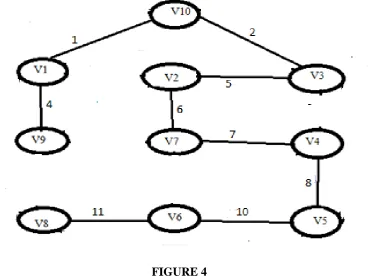
[image:8.595.125.494.312.591.2]According to step-4 of the algorithm, above selected edges are connected as shown in Figure 4.
FIGURE 4
Now applying step-5, it is found that the sub graph obtained at step-4, is a connected. Here, there are
two one degree vertices (Figure-9) and connecting these two vertices according to the step 6, the
Hamiltonian circuit is obtained as shown in Figure 5. Here step-8 to 13 are not involved.
GE-INTERNATIONAL JOURNAL OF ENGINEERING RESEARCH
VOLUME -2, ISSUE -4 (JUNE 2014) ISSN: (2321-1717)
FIGURE 5
The least cost Hamiltonian circuit is V1→V10 →V3 →V2 →V7 →V4 →V5 →V6 →V8 →V9 →V1
and the total cost = 1 + 2+ 5 + 6 + 7 + 8 + 10 + 11 + 12 + 4 = 66.
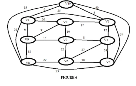
Experimental Result: [2]. Let us consider the graph of Figure 6 for m=1.
GE-INTERNATIONAL JOURNAL OF ENGINEERING RESEARCH
VOLUME -2, ISSUE -4 (JUNE 2014) ISSN: (2321-1717)
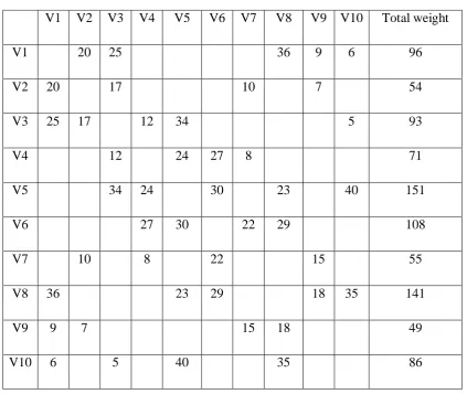
[image:10.595.94.518.138.495.2]The cost matrix of the graph and as per step-1, total weight of each vertex is calculated in table 2.
TABLE 2
V1 V2 V3 V4 V5 V6 V7 V8 V9 V10 Total weight
V1 20 25 36 9 6 96
V2 20 17 10 7 54
V3 25 17 12 34 5 93
V4 12 24 27 8 71
V5 34 24 30 23 40 151
V6 27 30 22 29 108
V7 10 8 22 15 55
V8 36 23 29 18 35 141
V9 9 7 15 18 49
V10 6 5 40 35 86
According to the step-2, the vertices in descending order are V5, V8, V6, V1, V3, V10, V4, V7, V2,
V9 and as per step-3, the least cost edge for these vertices are A[1] = (V5, V8), A[2]= (V8, V9), A[3]=
(V6, V7), A[4]= (V1, V10), A[5]= (V3, V10), A[6]= (V10, V3), A[7]= (V4, V7), A[8]= (V7, V4),
GE-INTERNATIONAL JOURNAL OF ENGINEERING RESEARCH
VOLUME -2, ISSUE -4 (JUNE 2014) ISSN: (2321-1717)
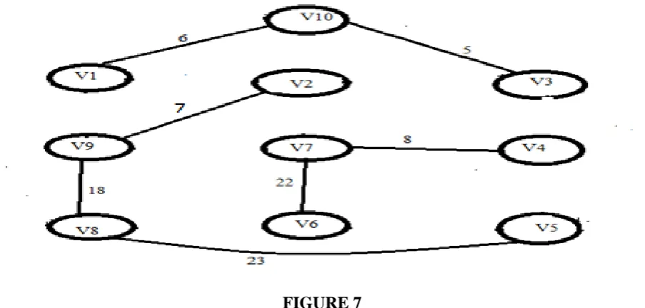
FIGURE 7
The sub-graph of Figure-7 above has three components (steps 5 & 4) and hence step-6 and step-7 are
not involved. Again step-9 and step-10 are also not involved here as there is no isolated vertex
according to step8. As per step-11, connectivity of one degree vertices are checked and it is found that
there is only one possible edge from vertex V1 and V6. Hence One possible edges (V1, V2) and (V6,
V5) are connected. There after the one possible edge (V4, V3) is generated and it is connected. Finally
it is found that there is no one degree vertex remained and hence goes to step-14. The least cost
Hamiltonian path is V1→V2 →V9 →V8 →V5 →V6 →V7 →V4 →V3 →V10 →V1 and total cost of
[image:11.595.82.540.520.752.2]the route is 20 + 7 + 18 + 23 + 30 + 22 + 8 + 12 + 5 + 6 = 151 ( step-14). The circuit is shown in
Figure 8.
FIGURE 8
GE-INTERNATIONAL JOURNAL OF ENGINEERING RESEARCH
VOLUME -2, ISSUE -4 (JUNE 2014) ISSN: (2321-1717)
FIGURE 9
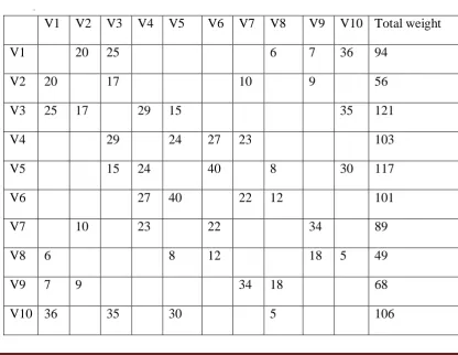
The cost matrix of the graph and as per step-1, total weight of each vertex is calculated in table 3.
TABLE 3
V1 V2 V3 V4 V5 V6 V7 V8 V9 V10 Total weight
V1 20 25 6 7 36 94
V2 20 17 10 9 56
V3 25 17 29 15 35 121
V4 29 24 27 23 103
V5 15 24 40 8 30 117
V6 27 40 22 12 101
V7 10 23 22 34 89
V8 6 8 12 18 5 49
V9 7 9 34 18 68
[image:12.595.94.511.436.758.2]GE-INTERNATIONAL JOURNAL OF ENGINEERING RESEARCH
VOLUME -2, ISSUE -4 (JUNE 2014) ISSN: (2321-1717)
As per step-2,the vertices in descending order are V3, V5, V10, V4, V6, V1, V7, V9, V2, V8 and as
per step-3, the least cost edge for these vertices are A[1]= (V3, V5), A[2]= (V5, V8), A[3]= (V10,
V8), A[4]= (V4, V7), A[5]= (V6, V8), A[6]= (V1,V8), A[7]= ( V7, V2), A[8]= (V9, V1), A[9]=
(V2, V9), A[10]= (V8, V10).
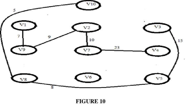
[image:13.595.117.507.215.432.2]According to step-4, the connections of these edges are shown below in Figure 10.
FIGURE 10
As per step-5, studying the components it is found that the sub graph obtained at step-4, is a
disconnected one. Hence step-6 and 7 are not involved. As per step -8, it is found that vertex V6 is
isolated one. Hence step-9 is involved. Now as per step-9, case-(c), least cost edge (V6, V8) with
weight 12 is connected, then degree of V8 becomes 3 and the weight of the newly connected edge is
greater than the weight of the previously connected edge hence edge (V6, V8) gets deleted. Again next
lesser weighted edge (V6, V7) with weight 22 is considered. As per step-9, case-(b), edge (V6, V7) is
connected and degree of vertex V7 became 3 and hence higher weighted edge (V7, V4) gets deleted.
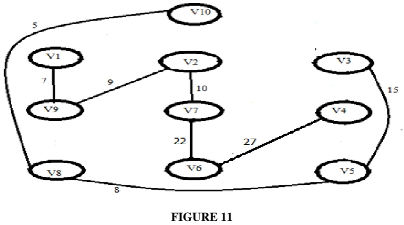
Again vertex V4 became isolate and step-9 is repeated. Edge (V4, V6) is connected. The new sub
GE-INTERNATIONAL JOURNAL OF ENGINEERING RESEARCH
VOLUME -2, ISSUE -4 (JUNE 2014) ISSN: (2321-1717)
FIGURE 11
As per step-10, lesser weighted edge from one degree vertices is checked and the lesser weighted
edge (V1, V8) is connected and the edge (V8, V5) gets deleted. The new sub graph thus obtained is
shown in Figure 12.
FIGURE 12
Now as per step-11, one possible edge among one degree vertices are checked and it is not found and
hence step-12 is involved. As per step-12, it is found that there is no connectivity problem and hence
highest weight one degree vertex V3 is connected with the next possible edge (V3, V4). Now one
possible edge (V10, V5) between one degree vertices is generated and hence step-11 is involved again.
[image:14.595.111.502.425.639.2]step-GE-INTERNATIONAL JOURNAL OF ENGINEERING RESEARCH
VOLUME -2, ISSUE -4 (JUNE 2014) ISSN: (2321-1717)
14 is involved and it is stopped. The least cost Hamiltonian path is V1→V9 →V2 →V7 →V6 →V4
→V3 →V5 →V10 →V8 →V1 and total cost of the route is 7 + 9 + 10 + 22 + 27 + 29 + 15 + 30 + 5 +
[image:15.595.107.502.159.398.2]6 = 160. The circuit is shown in Figure 13.
FIGURE 13
[image:15.595.95.512.443.690.2]Experimental Result: [4]. Let us consider the graph of Figure 14 for m = 1.
FIGURE 14
The cost matrix of the graph and the total weight of each vertex is calculated in table 4 as per step-1.
GE-INTERNATIONAL JOURNAL OF ENGINEERING RESEARCH
VOLUME -2, ISSUE -4 (JUNE 2014) ISSN: (2321-1717)
V1 V2 V3 V4 V5 V6 V7 V8 V9 V10 Total weight
V1 20 25 24 7 36 112
V2 20 17 10 40 87
V3 25 17 8 15 35 100
V4 8 6 27 23 64
V5 15 6 9 29 30 89
V6 27 9 22 34 92
V7 10 23 22 12 67
V8 24 29 34 18 5 110
V9 7 40 12 18 77
V10 36 35 30 5 106
As per step-2, the vertices in descending order are V1, V8, V10, V3, V6, V5, V2, V9, V7, V4 and as
per step-3, the least cost edge for these vertices are A[1]= (V1, V9), A[2]= (V8, V10), A[3]= (V10,
V8), A[4]= (V3, V4), A[5]= (V6, V5), A[6]= (V5, V4), A[7]= (V2, V7), A[8]= (V9, V1), A[9]= (V7,
[image:16.595.100.499.503.696.2]V2), A[10]= (V4, V5) . Now as per step-4, connection of these edges is shown in Figure 15.
FIGURE 15
As per step-5, it is found that the sub graph obtained at step-4 is a disconnected one and hence step-6
GE-INTERNATIONAL JOURNAL OF ENGINEERING RESEARCH
VOLUME -2, ISSUE -4 (JUNE 2014) ISSN: (2321-1717)
are not involved here. As per step-11, there is no one possible edge and hence step-12 is involved. As
per step-12, it is found that there is no connectivity problem and hence highest weighted one degree
vertex V1 is connected with next possible least cost edge (V1, V2). And it is found that one possible
edges (V3, V10), (V9, V8) and (V7, V6) are generated and hence step-11 is involved.
At step-11, all the one possible edges are connected and then it is found that there is no one
degree vertex and then step-14 is involved and stop. The least cost Hamiltonian path is V1→V9 →V8 →V10 →V3 →V4 →V5 →V6 →V7 →V2 →V1 and total cost of the route is 7 + 18 + 5 + 35 + 8 + 6
[image:17.595.86.506.270.482.2]+ 9 + 22 + 10 + 20 = 140. The circuit is shown in Figure 16.
FIGURE 16
GE-INTERNATIONAL JOURNAL OF ENGINEERING RESEARCH
VOLUME -2, ISSUE -4 (JUNE 2014) ISSN: (2321-1717)
FIGURE 17
The cost matrix of the graph and the total weight of each vertex is calculated in table 5 as per step-1.
TABLE 5
V1 V2 V3 V4 V5 V6 V7 V8 V9 V10 Total weight
V1 20 15 9 35 36 115
V2 20 17 30 40 107
V3 15 17 8 25 7 72
V4 8 6 27 23 64
V5 25 6 24 29 10 94
V6 27 24 22 34 107
V7 30 23 22 12 87
V8 9 29 34 18 5 95
V9 35 40 12 18 105
[image:18.595.99.509.421.725.2]GE-INTERNATIONAL JOURNAL OF ENGINEERING RESEARCH
VOLUME -2, ISSUE -4 (JUNE 2014) ISSN: (2321-1717)
As per step-2, the vertices in descending order are V1, V2, V6, V9, V8, V5, V7, V3, V4, V10 and as
per step-3, lesser weighted edges are assigned to these vertices are A[1]= (V1, V8), A[2]= (V2, V3),
A[3]= (V6, V7), A[4]= ( V9, V7), A[5]=(V8, V10), A[6]= (V5, V4), A[7]= (V7, V9), A[8]= (V3,
V10), A[9]= (V4, V5), A[10]= (V10, V8) .
[image:19.595.68.542.531.754.2]As per step-4, edges are connected as shown in Figure 18.
FIGURE 18
As per step-5, studying the sub graph it is found that the sub graph is disconnected one and hence step
6 is not involved. As per 8, there is no isolated vertex and hence step -11 is involved. As per
step-11, one possible edge (V6, V5) is connected. As there became one more one possible edge (V9, V1)
and it is connected. One degree vertices are remained and hence step-12 is involved. The new sub
GE-INTERNATIONAL JOURNAL OF ENGINEERING RESEARCH
VOLUME -2, ISSUE -4 (JUNE 2014) ISSN: (2321-1717)
FIGURE 19
As per step-12, it is found that there is connectivity problem between V2 & V10 and hence step-13 is
involved. As per step-13, case-(a), case-(ii) highest weight one degree vertex V2 is connected with
next lesser weight edge (V1, V2) and higher weight edge (V1, V9) gets deleted. And then step-11 is
involved. As there is no one possible edge and hence step-12 is involved. The new sub graph is shown
[image:20.595.75.529.231.420.2]in the Figure 20.
FIGURE 20
As per step-12, it is found that there is connectivity problem and hence step-13 is involved. According
to step-13, case-(a), case-(ii), highest weight one degree vertex V9, does not have lesser weighted edge
and lesser weighted edge (V10, V3) is connected and due to this edge degree of the vertex V3 became
3 and hence higher weighted edge (V3, V2) gets deleted. And the one possible edge (V9, V2) is
connected. The least cost Hamiltonian route is V1 → V2 → V9 → V7 → V6 → V5 → V4 → V3 →
V10 → V8 → V1 and the cost of the path is = 5 + 9 + 20 + 40 + 12 + 22 + 24 + 6 + 8 + 7 = 153 After
GE-INTERNATIONAL JOURNAL OF ENGINEERING RESEARCH
VOLUME -2, ISSUE -4 (JUNE 2014) ISSN: (2321-1717)
FIGURE 21
[image:21.595.83.522.356.609.2]Experimental Result: [6]. Let us consider the graph of Figure 22 for m=1.
FIGURE 22
The cost matrix of the graph and as per step-1, total weight of each vertex is calculated in table 6.
TABLE 6
V1 V2 V3 V4 V5 V6 V7 V8 V9 V10 Total weight
[image:21.595.78.522.685.756.2]GE-INTERNATIONAL JOURNAL OF ENGINEERING RESEARCH
VOLUME -2, ISSUE -4 (JUNE 2014) ISSN: (2321-1717)
V2 20 17 30 9 76
V3 15 17 8 25 7 72
V4 8 6 27 23 64
V5 25 6 24 29 35 119
V6 27 24 22 5 107
V7 30 23 22 36 78
V8 40 29 5 18 34 126
V9 10 9 36 18 73
V10 12 7 35 34 88
As per step-2, the vertices in descending order are V8, V5, V6, V1, V10, V7, V2, V9, V3, V4 and
as per step-3, lesser weighted edges are connected to these vertices are A[1]= (V8, V6), A[2]= (V5,
V4), A[3]= (V6, V8), A[4]= (V1, V9), A[A5]= ( V10, V3), A[6]= (V7, V6), A[7]= (V2, V9),
A[8]= (V9, V2), A[10]= (V3, V10), A[11]= (V4, V5).
[image:22.595.109.519.478.673.2]As per step-4, edges are connected as shown in Figure 23
FIGURE 23
As per step-5, it is found that the sub graph obtained at step-4, is a disconnected one and hence step-6
is not involved. As per step-8, it is found that there is no isolated vertex and hence step-9 & step-10
GE-INTERNATIONAL JOURNAL OF ENGINEERING RESEARCH
VOLUME -2, ISSUE -4 (JUNE 2014) ISSN: (2321-1717)
connected. Next one possible edge (V5, V8) is connected and then one possible edge (V1, V10) is
connected. As there is no one degree vertex remains hence step-14 is involved and it is stopped. Final
Hamiltonian circuit is shown in Figure 24. The least cost Hamiltonian route is
V1→V9→V2→V7→V6→V8→V5→V4→V3→V10→V1 and the cost of the path is = 12 + 10 + 9 +
[image:23.595.93.529.202.410.2]30 + 22 + 5 + 29 + 6 + 8 + 7 = 138.
FIGURE 24
Experimental Result: [7]. Let us consider the graph of Figure 25 and the structure of the graph is G
[image:23.595.86.527.477.706.2](3m + 7, 6m + 16) , when m=2.
FIGURE 25
GE-INTERNATIONAL JOURNAL OF ENGINEERING RESEARCH
VOLUME -2, ISSUE -4 (JUNE 2014) ISSN: (2321-1717)
TABLE 7
V1 V2 V3 V4 V5 V6 V7 V8 V9 V10 V11 V12 V13 Total
V1 - 2 22 28 5 12 69
V2 2 - 23 8 7 40
V3 22 23 14 16 17 92
V4 8 7 13 29 57
V5 14 7 25 15 61
V6 28 7 13 10 58
V7 5 10 3 22 21 61
V8 29 3 4 11 47
V9 25 4 26 20 75
V10 15 26 27 9 77
V11 11 20 27 1 59
V12 16 22 9 1 6 54
V13 12 17 21 6 56
As per step-2, the vertices in descending order are V3, V10, V9, V1, V5, V7, V11, V6, V4, V13,
V12, V8, V2 and as per step-3, the least cost weighted edges are assigned to these vertices are A[1]=
(V3, V5), A[2]= (V10, V12), A[3]= (V9, V8), A[4]= (V1, V2), A[5]= (V5, V4), A[6]= (V7, V8),
A[7]= (V11, V12), A[8]= (V6, V2), A[9]= (V4, V5), A[10]= (V13, V12), A[11]= (V12, V11),
GE-INTERNATIONAL JOURNAL OF ENGINEERING RESEARCH
VOLUME -2, ISSUE -4 (JUNE 2014) ISSN: (2321-1717)
FIGURE 26
As per step-5, it is found that the sub graph obtained at step-4, is a disconnected one and hence step-6
& 7 are not involved. As per step-8, it is found that there is isolated vertex and hence step-9 is
involved. As per step-9, case (b), isolated vertex V13 is connected with the least cost edge (V13, V12)
and the degree of the vertex V12 has become 3 and hence higher weighted edge (V12, V10) gets
deleted. Now vertex V10 has become isolated vertex and step-9, is repeated again. As per step-9,
case-(c), the least cost edge (V10, V12) cannot be connected and hence next lesser weighted edge (V10,
V9) is connected as per case-(a). After simplification the new sub graph is shown in Figure 27.
FIGURE 27
As per step-10, one degree vertices are examined and it is found that there is no lesser weighted edge
remained to connect and hence step-11 is involved. As per step-11, one degree vertices are examined
for one possible edge and it is found that there are two one possible edges (V4, V6) and (V11, V10).
These two edges are connected and then one more one possible edge (V3, V10) is generated and it is
connected. After this one more one possible edge (V1, V7) is generated and it is connected. Finally
there is no one degree vertex remained and hence step-14 is involved and stopped. The final least cost
[image:25.595.98.504.419.592.2]GE-INTERNATIONAL JOURNAL OF ENGINEERING RESEARCH
VOLUME -2, ISSUE -4 (JUNE 2014) ISSN: (2321-1717)
FIGURE 28
The least cost route is V1→V7→V8→V9→V10 →V11 →V12 →V13 →V 3 →V5 →V4→V6 →V2 →V1 with cost 17 + 6 + 1 +27 + 26 + 4 + 3 + 5 + 2 + 7 + 13 + 7 + 14 = 132.
5. CONCLUSION
This paper explains only an algorithm which will be more applicable for the particular type of graph in
solving traveling salesman problem.
REFERENCES
1. Karp M. R.,” Reducibility among combinatorial problems”, In R. E. Miller and J. W. Thatcher,
editors, Complexity of Computer Computations, Plenum Press, 1972, pp.-85-103.
2. Bora, K. C. and Kalita B, “Exact Polynomial-time Algorithm for the Clique Problem and P = NP for
Clique Problem”, International Journal of Computer Application, June 2013, Volume 73, No.8,
pp.-19-23.
3. Singh Anshul, Narayan Devesh, “A Survey Paper on Solving Travelling Salesman Problem Using
Bee Colony Optimization”, International Journal of Emerging Technology and Advanced
Engineering, May 2012, Issue 5, Volume 2, pp.-309-314.
4. Yadlapalli S., et al, “A Lagrangian-based Algorithm for a Multiple Depot, Multiple Traveling Salesman Problem”, Nonlinear Analysis: Real World Applications, Volume 10(4), 2009,
pp.1990-1999.
GE-INTERNATIONAL JOURNAL OF ENGINEERING RESEARCH
VOLUME -2, ISSUE -4 (JUNE 2014) ISSN: (2321-1717)
6. Hlaing Zar Chi Su Su and Khine May Aye,”Solving Traveling Salesman Problem by Using Improved Ant Colony Optimization Algorithm”, International Journal of Information and Education
Technology, Vol. 1, No.5, December 2011, pp.404-409.
7. Kumbharana Sharad N. and Pandey Gopal M., ”Solving Travelling Salesman Problem using
Firefly Algorithm”, International Journal for Research in Science & Advanced Technologies, Vol. 2,
Issue 2, 2013, pp.53-57.
8.Dutta Anupam, et al, “Regular Planar Sub-Graphs of Complete Graph and Their Application”,
International Journal of Applied Engineering Research ISSN 0973-4562, Volume 5, Number 3 (2010)
pp 377-386.
9. Ahmadvand Mohammad et. al.,”Solving the Traveling Salesman Problem by an Efficient Hybrid Metaheuristic Algorithm”, Journal of Advances in Computer Research, Vol. 3, No. 3, August 2012,
pp.75-84.
10. Sallabi Omar M., El-Haddad Younis, “An Improved Genetic Algorithm to Solve the Traveling Salesman Problem”, World Academy of Science, Engineering and Technology, Volume 52, 2009,
pp.471-474.
11. Bora, K. C., Kalita, B.,” Particular Type of Hamiltonian Graphs and Their Properties”,
International Journal of Computer Application, to appear.
12. Kalita, B., “Sub-Graphs of Complete Graph”, Proc. International Conference of Foundation of
Computer Science |FCS’06|, Las Vegus, USA, pp.71-77.2006.
13. Choudhury, Jayanta Kr. and Kalita, B., “An Algorithm for Traveling Salesman Problem”, Bulletin
of Pure and Applied Sciences, Volume 30 E (Math & Stat.) Issue (No.1)2011: pp.- 111-118.
14. Dutta, Anupam. et al, “Regular sub-graph of Complete Graph”, International Journal of Applied
Engineering Research, Volume 5, Number 8, 2010, pp.1315-1323.
15. Choudhury, Jayanta Kr. et al, “Graph Factorization And Its Application”, International Journal of
Management, IT and Engineering”, Volume 2, Issue 3, March 2012, pp.208-220.
16. Choudhury, Jayanta Kr. et al, “Decomposition of Complete Graphs into Circulant Graphs and its Application”, International Journal of Computer Engineering and Technology, Volume 4, Issue 6,
November – December (2013), pp.25-47.