The evolution of dust emitted by a uniform source above ground level

PII. S0161171203106163 http://ijmms.hindawi.com © Hindawi Publishing Corp.

THE EVOLUTION OF DUST EMITTED BY A UNIFORM

SOURCE ABOVE GROUND LEVEL

I. A. ELTAYEB and M. H. A. HASSAN

Received 18 June 2001 and in revised form 21 January 2002

A uniform source situated at a fixed location starts to emit dust at a certain time, t=0, and maintains the same action fort >0. The subsequent spread of the dust into space is governed by an initial boundary value problem of the atmospheric diffusion equation. The equation has been solved when the wind speed is uniform and diffusion is present both along the vertical and the horizontal for a general source. The solution is obtained in a closed form. The behaviour of the solution is illustrated by means of two examples, one of which is relevant to industrial pollution and the other to the environment. The solution is represented in graphic form. It is found that the spread of dust into space depends mainly on the type of source and on the horizontal component of diffusion. For weak diffusion, the dust travels horizontally with a vertical front at the uniform speed of the flow. In the presence of horizontal diffusion, dust diffuses vertically and horizontally. For a point source, the distribution of dust possesses a line of extensive pollution. For a finite-line source, the dust concentration possesses a point of accumulation that moves both horizontally and vertically with time.

2000 Mathematics Subject Classification: 35K15, 35Q35, 49K20, 35C15.

The transport of such dust particles is usually governed by the atmospheric diffusion equation

∂c∗

∂t∗+u·∇c∗= ∇·

D·∇c∗−w·∇c∗, ∇·u=0 (1.1)

in whichu is the wind velocity,wis the settling velocity, andDis the stress tensor. The settling velocity depends on the particle size and can be taken as a measure of the influence of gravity. The stress tensor is a function of position and its dependence in different directions may be different so that it is not isotropic. The velocity, in general, depends on the position as well as time. The second term on the left-hand side of the first equation in (1.1) represents the advection of the particles by the local fluid motion.

The atmospheric diffusion equation has been solved in a variety of situa-tions (see, e.g., [2,11,12,13]). In all these cases, the stress tensor and velocity were assumed to take reasonably simple forms, with the most complicated forms being when one or both varied as a power law of the vertical coordinate. The reason for this is that complicated forms pose equations which cannot be solved analytically. Since the domain of influence of velocity on dust particles of interest is quite small, in terms of atmospheric dimensions, these simple forms are adequate since they can be considered as first terms in Taylor series expansions for these functions.

We will assume that the stress tensor has the form

D=    

γ 0 0

0 0 0

0 0 λz∗   

 (1.2)

in whichγandλare constants, and the flowuis unidirectional and uniform so that

u=(U,0,0), w=(0,0,W ) (1.3)

in a Cartesian system of coordinates in which thez-axis is directed vertically upwards and thex-axis along the horizontal wind speed.

Most previous studies have concentrated on the steady-state solution of the diffusion equation (1.1). One of our interests here is to examine how such a steady state can be achieved. This requires the consideration of an initial boundary value problem in which case the time derivative is fully potent so that the equation is predictive. This allows us to examine the dependence of the solution on the initial conditions with a view to identifying the manner in which the steady-state solution is achieved. For this reason, we will consider a situation for which the steady-state solution is known [6].

InSection 2, we define the initial value problem and boundary conditions. In

...

simplified solutions for them. We also examine the case when time increases indefinitely and obtain a limiting solution which matches the already known solution of the steady-state problem. InSection 4, we examine the solution in detail and illustrate its dependence on the parameters of the problem as it evolves with time.Section 5is devoted to a few concluding remarks.

2. Formulation of the problem. Consider a source atx=0 emitting dust at a prescribed (measured) rate. Such a situation may arise when dust passing through a certain position is measured at various levels. We intend to examine the development of the distribution of dust with time until a steady state is reached. Define a Cartesian system of coordinatesO(x∗,y∗,z∗)in whichOz∗

is vertically upwards and Ox∗ and Oy∗ are horizontal. The concentration

c(x∗,z∗,t∗) of pollutant particles is governed by (1.1), (1.2), and (1.3). We assumed that the concentration is independent of the lateral coordinatey∗, and depends on the timet∗. Thus (1.1) takes the form

∂c∗ ∂t +U

∂c∗ ∂x∗ =

∂ ∂x∗γ

∂c∗ ∂x∗+

∂ ∂z∗λz

∂c∗ ∂z∗+W

∂c∗

∂z∗, (2.1)

whereU,W ,γ, andλare defined in (1.2) and (1.3). If we define

b=γ λ

λ U

2

, ν=₂W

λ, x= λ U

x∗, t∗= t

λ, z=z

∗_{, (2.2)}

we can write (2.1) in the neat form

∂c∗ ∂t +

∂c∗

∂x =(2ν+1)z ∂c∗

∂z + ∂2_c∗

∂z2 +b

∂2_c∗

∂x2. (2.3)

This equation is solved subject to boundary and initial conditions. Since the source is switched on at a certain time, we will assume that the concentration vanishes everywhere for t≤0. The distribution of the concentration can be assumed to satisfy one or more conditions at the ground level. We will assume here that the concentration vanishes at the top of the roughness layer,z=zo. Another possible condition is the vanishing of the flux, which demands that

∂c∗/∂z=0 atz=zo. However, the imposition of the latter boundary condition will render the inversion of the transforms encountered in the solution more difficult. Since the subsequent distribution of the dust is entirely due to the emission by the source atx=0, we can impose the condition that it decays to zero faraway fromx=0. The initial condition can be written in the form

in which the Heaviside function is defined by

H(x−a)=   

1 forx > a,

0 forx < a, (2.5)

andf (z)is an arbitrary function representing the variation of the source with height whileQmeasures the amplitude of the source.

If we define

q(x,ς,t)=ςν_{c(x,ς,t), ς=2z}1/2_{, c=Qc}∗_{, (2.6)}

we can rewrite (2.3) as

∂q ∂t+

∂q ∂x=

1

ς ∂ ∂ς ς

∂q ∂ς

−ν2

ς2q. (2.7)

If we make the further transformation

u(x,ς,t)=e−x/2b_{q(x,ς,t), (2.8)}

we obtain

∂u ∂t =

1

ς ∂ ∂ς ς

∂u ∂ς

−ν2

ς2u+b

∂2_u

∂x2−

1

4bu. (2.9)

The boundary and initial conditions can also be transformed tou:

ux,ς0,t

=0, (2.10a)

c(x,ς,t)→0 asς → ∞, (2.10b)

u(0,ς,t)=H(t)f ς

2

4

, (2.10c)

u(x,ς,0)=0 ∀x,ς≥0. (2.10d)

We are therefore required to solve (2.9) subject to the initial boundary condi-tions (2.10).

3. The solution. The solution is obtained by adopting the Weber transform defined by

˜

q(x,y,p)= _∞

zo

q(x,y,z)Hν(pz)z dz, (3.1)

in which

Hν(pz)=Jν(pz)Yν

pzo

−Jν

pzo

Yν(pz), (3.2)

together with its inverse transform

q(x,y,z)= _∞

0

˜

q(x,y,p)Hν(pz) Jν2pzo

+Yν2pzo

...

In (3.2),Jν(x)and Yν(x)are Bessel functions of the first and second kinds with orderνand argumentx.

If we apply the transform (3.1) to (2.9), we get

∂u¯

∂t =b ∂2_u¯

∂x2− p 2₊ 1

4b

¯

u. (3.4)

By taking the Laplace transform of (3.4) in time and using (2.10d), we find that

su(x,p,s)ˆ¯ =b∂

2_uˆ¯

∂x2− p 2₊ 1

4b

ˆ ¯

u. (3.5)

If we apply both transforms to (2.10c) in the same order, we obtain

ˆ ¯

u(0,p,s)=F(p)1

s (3.6)

in which

F(p)= ∞

ς0

f ς

2

4

Hν(pς)ςν+1dς. (3.7)

Equation (3.5) can be solved together with (2.10d) and (3.6) to find that

ˆ ¯

u(x,p,s)=F(p)1 sexp

−as+c2_{, a=}√x

b, c=

p2₊ 1

4b. (3.8)

The next step is to invert the two transforms. Inverting the Laplace transform intgives

¯

u(x,p,t)=F(p)G(x,t;p), (3.9)

whereG(x,t;p)is obtained by the use of a combination of shift and convolu-tion theorems. Thus

G(x,p,t)= x

2√πb t

0τ

−3/2_{exp −c}2

τ− x

2

4bτ

dτ

= x

2√πbt ∞

1

1

√ vexp

ctt v2−

xv

4bt

dv.

(3.10)

This solution can best be expressed as a combination of complementary error functions in order to make use of the asymptotic properties of these well-known functions. Hence

G(x,p,t)

=1₂

exp(−ac)erfc

₁

2xt −1/2₋

ct1/2

+exp(ac)erfc

₁

2xt

−1/2_+ct1/2

,

in which erfc(x)is the standard complementary error function with argument

x(see, [1, page 295]).

The closed form of the solution is obtained by inverting (3.9) using (3.3). Thus

u(x,ς,t)= ∞

0

F(p)Hν(pς)G(x,p,t) Jν2pς0+Yν2pς0 p dp,

(3.12)

c(x,ς,t)=ς−νexp x 2b

∞

0

Hν(pς)F(p) Jν2pς0

+Yν2pς0

G(x,p,t)p dp. (3.13)

The functionF(p)must be found while its inverse is known, but the use of its inverse means the use of the convolution theorem for the Weber transform. In general, this leads to a rather complicated double integral. However, the result-ing integral can be reduced to an integral in one variable for certain forms of the functionf (z). We will illustrate this by two examples discussed in Sections

4and5.

4. Uniform point source. When the source at x=0 is concentrated at a point z=h (i.e., f (z)=δ(z−h)) above ground level, the expression F(p)

reduces to

F(p)=hν+0 1, h0=2h1/2. (4.1)

The problem posed here is relevant to industrial pollution where a chimney emits a pollutant into the surrounding environment.

The expressions (3.12) and (3.13) here reduce, respectively, to

u(x,ς,t)= ∞

0

Hν(pς)Hν

ph0

J2

νpς0+Yν2pς0G(x,t

;p)p dp, (4.2)

c(x,ς,t)=h0ν+1ς−νexp x

2b ∞

0

Hν(pς)Hνph0

J2

νpς0+Yν2pς0G(x,t

;p)p dp.

(4.3)

The relatively simple solution (4.3) can be used to examine a number of limiting cases which may clarify the manner in which time variations influence the distribution of dust.

Special limiting cases. _{Here, we examine the general solution (3.13) in} special cases where the solution is simpler and reduces to situations studied previously.

...

for very large times. Now, (3.11) gives

G(x,p,t)≈e−acerfc−ct1/2_+eac_erfcct1/2 _{fort → ∞. (4.4)}

If we use the reflection property of the error function

erfc(−z)=2−erfc(z), (4.5)

we obtain

f (x,t;p)≈2e−ac+2 sinh(ac)erfcct1/2_≈2e−ac _{fort → ∞ (4.6)}

and the solution (4.3) reduces to

c(x,ς,t)

=hν+1

0 ς−νexp ₂x

b ∞

0

Hν(pς)Hν

ph0

J2

ν

pς0

+Y2

ν

pςo

exp −₂x b

1+4bp2

p dp

(4.7)

which is identical to [6, (3.12)] for the steady-state solution. (ii)t→0. Whentis very small, we have

G(x,p,t)≈e−acerfc 1 2at

−1/2

+eac_erfc 1 2at

−1/2

≈2 cosh(ac)erfcct−1/2.

(4.8)

Here, we appeal to the asymptotic property of the error function

erfc(z)≈(πz)−1/2exp−z2

1+ ∞

n=1

(−1)n1·3···( 2n−1)

2z2n

, |z|→ ∞,

|argz| ≤π₂−δ, δ >0,

(4.9)

to find thatc(x,ς,t)becomes zero astvanishes.

3 2.5 2 1.5 1 0.5 x 0 2 4 6 8 10 12 14 z 0.285 0.951 0.476 0.0951 (a) 10 8 6 4 2 x 0 2 4 6 8 10 12 14 z 0.38 0.856 0.285 0.0951 0.19 (b) 10 8 6 4 2 x 0 2 4 6 8 10 12 14 z 0.19 0.285 0.0951 0.38 0.951 (c) 10 8 6 4 2 x 0 2 4 6 8 10 12 14 z 0.19 0.285 0.0951 0.38 _0.951 0.856 (d)

Figure_4.1. _{The isolines of the concentration of the point source in} the(x,z)plane whenh=5.0,ν=0.5, andzo=0.5 for (a)t=1.5, (b)t=5.0, (c)t=9.0, and (d)t=50.0, in the case when there is no horizontal diffusion.

function leads to

G(x,p,t)≈x √

bt √

2π exp

−x2+t2

4bt

→0 asb →0 (4.10)

but in case (iiib), we use both properties (4.5) and (4.9) of the error function to find that

f (x,t;p)≈exp

−xp2₋ x

2b +x √ bt √

2π exp

−x2+t2

4bt

asb →0. (4.11)

The solution in the caseb=0 then has the form

c(x,ς,t)=hν+0 1ς−νH(t−x)

_∞

0

Hν(pς)Hν

ph0

Jν2pς0

+Yν2pς0

e−xp2p dp (4.12)

...

5. Vertical source of finite length. Consider a source situated alongx=0 such that (see (2.10c))

f (z)=   

1 forzo< z < L,

0 forz > L, (5.1)

so that the pollutant is emitted uniformly throughout the distance between the heightsz=zoandz=Lalong the vertical linex=0. This situation is of great relevance to the spread of dust in arid and semiarid lands where desertification is a major problem (see, e.g., [3]).

The solution is obtained by using the expression (5.1) into (3.7), (3.9), and (3.12). We find that

F(p)=Yνpς0I1−Jνpς0I2, (5.2)

in which

I1=

L

ς0

ςν+1Yν(pς)dς, I2=

L

ς0

ςν+1Jν(pς)dς. (5.3)

Forς0→0, these two integrals can be evaluated analytically (see [8, page 683]).

They reduce to

I1=

ν+1_J

ν+1(p )

p , I2=

ν+1_Y

ν+1(p )

p +

2ν+1_Γ(ν+1)

πpν+2 , (5.4)

in whichΓ(x)is the Gamma function of argumentx. It then follows that

pF(p)= ν+1 p

Yν(pς)Jν+1(p )−Jν(pς)Yν+1(p )

− 2ν+1

πpν+2Γ(ν+1). (5.5)

The integral (3.13) together with (5.5) has been computed for various values of the parametersν,L, andbin the(x,ς,t)space and a sample of the results is given in Figures6.5and6.6.

6. Discussion. The expression (3.13) for the concentrationc(x,ς,t)was in-tegrated numerically for the two cases of a point source (discussed inSection 4) and of a vertical uniform source (discussed inSection 5), for various values of the parameters. The results of the point source are presented in Figures4.1,

6.1,6.2,6.3, and6.4while those of the vertical source are illustrated in Figures

5 4 3 2 1

x 2

4 6 8 10 12 14

z 0.217

2.17 0.651 0.434

(a)

10 8 6 4 2

x 2

4 6 8 10 12 14

z

1.52 0.218

0.435

(b)

10 8 6 4 2

x 2

4 6 8 10 12 14

z

0.248

2.23

0.495

0.99

0.743

(c)

10 8 6 4 2

x 2

4 6 8 10 12 14

z

0.114

0.228 0.342

0.456 1.71

(d)

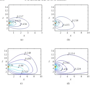
Figure_6.1. _{The isolines of the concentration of the point source} in the(x,z)plane whenh=5.0,ν=0.5,zo=0.5, andb=1.0 for (a)t=2.0, (b)t=5.0, (c)t=9.0, and (d)t=50.0. Compare with

Figure 4.1and note the influence of the horizontal diffusion.

...

0 2 4 6 8 10

z

x

1 2 3 4 5 6

0.217 0.434

0.651 1.95

(a)

0 2 4 6 8 10

z

x

1 2 3 4 5 6

0.215 0.645

0.43 1.93

(b)

0 2 4 6 8 10

z

x

1 2 3 4 5 6

0.201 0.401

0.602 1.8

(c)

0 2 4 6 8 10

z

1 2 3 4 5 6

x 0.2 0.399

0.599 1.6

(d)

Figure_6.2. _{The isolines of the concentration of the point source} for different sets of values of parameters illustrating the effects of the parametersh,ν,b, andzofor a fixed value of time,t=5.0. (a) h=5.0,ν=1.0,zo=0.5,b=1.0; (b)h=2.0,ν=1.0,zo=0.5, b=1.0; (c)h=5.0,ν=1.0,zo=0.5,b=3.0; (d)h=5.0,ν=1.0, zo=0.1,b=1.0.

Whereas the parameter representing horizontal diffusion provides a strong influence on the evolution of the dust with time, the remaining parameters play a more subservient role. The influence of the parametersh, ν, and zo is illustrated inFigure 6.2. Comparing Figures6.1(b) and 6.2(a), we see that the increase inν(representing an increase in the settling velocity and hence stronger gravitational effect) limits the spread of the dust above the source and tends to force it to settle to the ground. The increase in the height of the source enhances the spread of the dust in the horizontal direction since it allows the particles to acquire relatively higher velocities before they reach the ground, as can be seen by comparing Figures6.2(a)and6.2(b). The roughness height

Zc

0 1 2 3 4 5

1 2 3 4 5

x

(i), (ii)

(iii)

(iv)

(a)

Cc

0 0.2 0.4 0.6 0.8 1

1 2 3 4 5

x

(iii) (i)

(b)

Zc

0 1 2 3 4 5

x

2 4 6 8 10

(iv)

(i)

(ii)

(iii)

(c)

Cc

0 0.1 0.2 0.3 0.4 0.5

x

0 2 4 6 8 10

(i) (iii)

(iv)

(d)

Figure_6.3. _{An illustration of the dependence of the curve of} ex-tensive pollution, heightZc, and concentrationCc along it on the parameters of the point source problem. (a) and (b) correspond to t=5.0,h=5.0, and (i)zo=0.5,ν=0.5,b=2.0; (ii)zo=0.5,ν=0.5, b=3.0; (iii)zo=0.5,ν=1.5,b=2.0; and (iv)zo=0.1,ν=0.5, b=2.0, respectively. (c) and (d) again correspond toh=5.0, and (i) zo=0.5,ν=0.5,b=3.0,t=10.0; (ii)zo=0.5,ν=1.5,b=3.0, t=10.0; (iii)zo=0.1,ν=1.5,b=3.0,t=10.0; and (iv)zo=0.5, ν=0.5,b=3.0,t=50.0, respectively.

For all values of the parameterbin the case of a point source, the concen-tration of dust possesses a curve of extensive pollution. This is defined as the curve on which, for every value ofx, the concentration is maximized overz. The profile of this curve, which was identified in the steady-state solution [6], is here found to evolve with time, in addition to its dependence on the pa-rameters of the problem. This is illustrated in Figures6.3and6.4.Figure 6.3

...

Zc

0 1 2 3 4 5

x

2 4 6 8 10

(i), (ii), (iii)

(iv)

(v)

(a)

Cc

0 0.1 0.2 0.3 0.4

x

0 2 4 6 8 10

(iv)

(v)

(i), (ii), (iii)

(b)

Zc

0 1 2 3 4 5

x

2 4 6 8 10

(iii)

(ii) (i)

(iv)

(v)

(c)

Cc

0 0.1 0.2 0.3 0.4

x

2 4 6 8 10

0

(v) (i) (iv) _(ii)

(iii)

(d)

Figure_6.4. _{A sample of the data obtained for the curve of extensive} pollution of dust in the(x,z)plane for different values of time and two values ofbwhen the source is situated at one point; (a), (b) for b=0 and (c), (d) forb=3.0. Figures6.4(a)and6.4(c)represent the variations in height of the point with horizontal distancexwhile (b) and (d) represent the profiles of the concentration as a function ofxwhenh=5.0. The curves refer to the sets of data: (i)t=5.0, ν=0.5,zo=0.5, (ii)t=10.0,ν=0.5,zo=0.5, (iii)t=50.0,ν=0.5, zo=0.5, (iv)t=5.0, ν=1.5,zo=0.5, and (v)t=5.0, ν=0.5, zo=0.1.

N

0 0.5 1 1.5 2 2.5 3

x

0 1 2 3

0.082 0.164

0.41 0.656

0.82 0.82 0.246

(a)

N

0 0.5 1 1.5 2 2.5 3

x

0 1 2 3 4 5

0.0544 0.109

0.163

0.272 0.435

0.49

0.544 0.272

(b)

N

0 0.5 1 1.5 2 2.5 3

x

1 2 3 4 5

0

0.0329

0.0658

0.0988 0.23 0.296

0.329 0.165

(c)

N

0 0.5 1 1.5 2 2.5 3

x

1 2 3 4 5

0

0.00978 0.0196

0.0587 0.0782

0.0978 0.0391

0.0293

(d)

Figure_6.5. _{A sample of the results for the computation of the} ex-pression for the concentration of dust in the case of a finite vertical source whenν=0.5,b=0.5, andL=1.0 for different times: (a) t=1.0, (b)t=5.0, (c)t=10.0, and (d)t=20.0. Note the slow move-ment of the point of accumulation with increasing time.

inν andzo. The behaviour of the concentration on the curve is different. In the absence of horizontal diffusion, the concentration does not change with time (Figure 6.4(b), (i), (ii), (iii)). When horizontal diffusion is present, the curve is displaced downwards as it evolves with time (Figure 6.4(d), (i), (ii), (iii)). The changes due to the different parametersνandzoare small, as can be observed in Figures6.4(b)and6.4(d).

...

N

0 0.5 1 1.5 2 2.5 3

x

0 1 2 3 4 5

0.0544

0.109

0.272 0.544 0.435

0.272

(a)

N

0 0.5 1 1.5 2 2.5 3

x

1 2 3 4 5

0

0.12

0.2 0.4 0.32

0.04

0.24

(b)

N

0 0.5 1 1.5 2 2.5 3

x

0 1 2 3 4 5

0.0624 0.125 0.312 0.562

0.624

0.312

(c)

N

0 0.5 1 1.5 2 2.5 3

x

0 1 2 3 4 5

0.115 0.229

0.458

0.573 1.15

(d)

Figure_6.6. _{The contours of the concentration of dust for the} ver-tical source at a fixed time,t=5.0, for different sets of the param-eters: (a)ν=0.5,b=0.5,L=1.0, (b)ν=0.5,b=1.5,L=1.0, (c) ν=0.5,b=0.5,L=3.0, and (d)ν=2.0,b=0.5,L=1.0.

Figures6.6(a)and6.6(b)shows that the increase in horizontal diffusion (i.e., in

b) promotes the spread of dust and enhances the advance of the accumulation point. The increase in the extent of the source (i.e., inL) naturally promotes the spread of dust vertically while the increase in the settling velocity (i.e., in

ν) forces the dust to settle down to the ground, as can be seen inFigure 6.6(d).

that the most significant change in the solution is due to the presence of the horizontal component of diffusion. In its absence, the dust spreads into space in such a way that its front is vertical and has the uniform horizontal speed of the wind while it diffuses vertically. The presence of the horizontal com-ponent of diffusion destroys the sharp vertical nature of the advancing front and the dust diffuses ahead of the vertical line moving horizontally with the speed of the flow. Whether the horizontal diffusion is strong or weak, the dis-tribution of dust possesses a curve of extensive pollution which evolves in a manner dependent on the parameters of the problem but its height is weakly dependent on time as it extends in space with increasing time.

The behaviour of the solution for large times has been examined in detail with a view to assessing the manner in which a steady state is achieved. It was found that in the case of a point source, as time increases indefinitely, the solution uniformly approaches the steady-state solution obtained previously [6] by solving the equations in the absence of time variation.

The problem posed by a uniform vertical finite source was also discussed to illustrate the strong dependence of the solution on the type of source under consideration. It is found that the general influence of the parameters repre-senting the components of diffusion and settling velocity is very similar but the distribution of the dust in the(x,z)plane is drastically different.

References

[1] M. Abramowitz and I. A. Stegun (eds.),Handbook of Mathematical Functions, with Formulas, Graphs, and Mathematical Tables, National Bureau of Standards, Applied Mathematics Series, vol. 55, U.S. Government Printing Office, Dis-trict of Columbia, 1965.

[2] J. G. Bartzis,Turbulent diffusion modeling for wind flow and dispersion analysis, Atmospheric Environment23(1989), 1963–1969.

[3] H. E. Dregne,Desertification of arid lands, Physics of Desertification (F. El-Baz and M. H. A. Hassan, eds.), Martinus Nijhoff Publishers, Dordrecht, 1986, pp. 4–34.

[4] F. El-Baz, I. A. Eltayeb, and M. H. A. Hassan (eds.),Sand Transport and Desertifi-cation in Arid and Semi-Arid Lands, World Scientific Publishers, Singapore, 1990.

[5] I. A. Eltayeb and M. H. A. Hassan,On the non-linear evolution of sand dunes, Geophys. J. R. Astr. Soc.65(1981), 31–45.

[6] ,Diffusion of dust particles from a point source above ground level and a line source at ground level, Geophys. J. Internat.142(2000), 426–438. [7] D. A. Gillette,Threshold friction velocities for dust production for agricultural

soils, J. Geophys. Res.93(1988), 12645–12662.

[8] I. S. Gradshteyn and I. M. Ryzhik,Table of Integrals, Series, and Products, Aca-demic Press, New York, 1980.

[9] M. H. A. Hassan and I. A. Eltayeb,Suspension of transport of wind eroded sand particles, Geophys. J. Internat.104(1991), 147–152.

...

[11] J. S. Lin and L. Hildemann,A generalized mathematical scheme to analytically solve the atmospheric diffusion equation with dry deposition, Atmospheric Environment31(1997), 59–71.

[12] R. P. Llwelyn,An analytical model for transport, dispersion and elimination of air pollutants emitted from a point source, Atmospheric Environment17

(1983), 249–256.

[13] O. F. T. Roberts,The theoretical scattering of smoke in a turbulent atmosphere, Proc. Roy. Soc. London Ser. A104(1923), 640–654.

[14] R. A. Schmidt,Vertical profiles of wind speed, snow concentration, and humidity in blowing snow, Boundary-Layer Meteorol.23(1982), 223–246.

[15] M. Sharan, M. P. Singh, and A. K. Yadav,Mathematical model for atmospheric dis-persion in low winds with eddy diffusivities as linear functions of downwind distance, Atmospheric Environment30(1996), 1137–1145.

[16] E. L. Skidmore,Soil erosion by wind: an overview, Physics of Desertification (F. El-Baz and M. H. A. Hassan, eds.), Martinus Nijhoff Publishers, Dordrecht, 1986, pp. 261–273.

[17] M. Takeuchi,Vertical profile and horizontal increase of drift snow transport, J. Glaciol.26(1980), no. 94, 481–492.

I. A. Eltayeb: Department of Mathematics and Statistics, College of Science, Sultan Qaboos University, P.O. Box 36, Al-Khodh 123, Muscat, Sultanate of Oman

E-mail address:ieltayeb@squ.edu.om

M. H. A. Hassan: Third World Academy of Sciences, International Centre for Theoret-ical Physics, P.O. Box 586, Miramare 11, 34100 Trieste, Italy