Method for Multi attribute Decision Making with Triangular Fuzzy Number Based on Multi period State

(1)

Method for Multi-attribute Decision Making with

Triangular Fuzzy Number Based on Multi-period State

Sha Fu

Department of Information Management, Hunan University of Finance and Economics, China

Abstract

This paper takes the time weight and attribute weight in different periods into consideration to propose a dynamic triangular fuzzy number type multi-attribute decision making method to solve the problem with multi-attribute decision making with triangular fuzzy number as the attribute value. This method utilizes the characteristics of the triangular fuzzy number in order to establish the correlation model between the evaluation scheme and the positive and negative ideal scheme, and obtain comprehensive ranking of the evaluation scheme, thus acquiring the decision making result. At last, this paper demonstrates the feasibility and validity of the proposed methods through instance analysis.

Keywords

Multi-period, Triangular Fuzzy Number, Multi-attribute Decision Making, Time Weight Vector, Best Affiliate Degree

1. Introduction

Multi-attribute decision making is a very important component of modern decision science. It is also called finite scheme multi-objective decision. This theory and method have been widely used in engineering design, social life, economic system and management science and other fields since a long time ago. Multi-attribute decision making problems are of profound theoretical significance in various fields. Since it is widely used, researches about it have always been the focus of the major topics. In real life, due to limitation of the humans’ experience and knowledge and fuzziness of positive cognition, people’s cognition of things, especially things that are always undergoing constant changes and development, is uncertain, and cannot provide sufficient amount of information required for index evaluation and measurement in an accurate manner.

In real decision making, much information is both uncertain and fuzzy, which means that the comments of decision makers on the indexes can hardly be expressed with precision numerical numbers. In such a case, people

(2)

containing triangular fuzzy numbers, and designed the group information aggregation optimized model based on the two targets of individual evaluation value and group evaluation value, i.e., optimal distance and high similarity. Finally, he proposed an expansion VIKOR method. Huang and Luo [9] proposed the index weight measurement based on the triangular fuzzy number comparison possibility relation by referring to the related thoughts of maximized empowerment algorithm and the triangular fuzzy number comparison possibility theory, to solve the problem with UMADM with triangular fuzzy number as the index value. In addition, a comparison possibility degree relation method of triangular fuzzy number type UMADM is proposed to judge the advantages and disadvantages and order of the decision making scheme set. By comprehensive analysis of various literatures, the researches of various scholars mainly focus on the problems with triangular fuzzy number multi-attribute decision making in a single period. There have been only a few researches focusing on the problems with triangular fuzzy number multi-attribute decision making of multi-period or multi-stage. In practical application, for many complicated decision making problems, the original decision making information of various periods should be taken into consideration. For instance, the decision making information for multi-period investment decision making, and validity dynamics of medical diagnosis and military system should include the time dimension. For this reason, researches of dynamic multi-attribute decision making problems are of great theoretical significance and practical application value, and would hopefully become another hot research topic in the decision making science field.

2. Decision Making Criteria and

Methods

2.1. Triangular Fuzzy Number

Assume

a

ˆ

=

[

a

L

,

a

M

,

a

U

]

, where

₀

_<

_a

L

_≤

_a

M

_≤

_a

U

and

a

ˆ

is the triangular fuzzy number; the subordinate function could be expressed as follows:

   

    

 

> ≤ ≤ −

−

≤ ≤ −

−

<

= µ

U U M

U M

U

M L

L M

L

a

a x

a x a a a

a x

a x a a a

a x

x

, 0

, , , 0

) (

ˆ (1)

Where,

a

L and

a

U are respectively the lower limiting and upper limiting values of

a

ˆ

and

a

M is the mid-value.

Assume

a

ˆ

=

[

a

L

,

a

M

,

a

U

]

and

b

ˆ

=

[

b

L

,

b

M

,

b

U

]

are any two of the triangular fuzzy numbers. The algorithm is as follows:

1)

a

ˆ

+

b

ˆ

=

[

a

L

+

b

L

,

a

M

+

b

M

,

a

U

+

b

U

]

; 2)

a

ˆ

×

b

ˆ

=

[

a

L

b

L

,

a

M

b

M

,

a

U

b

U

]

; 3)

_{λ =}

_a

ˆ

[

_λ

_a

L

,

_λ

_a

M

,

_λ

_a

U

]

_,

_λ

_≥

₀

_;

4)

[

1 ,

1 ]

ˆ

1

L M

U

_a

a

=

,

a

L

,

a

M

,

a

U

≠

0

.

2.2. Distance and Grey Matrix of Triangular Fuzzy Number

Definition 1: Assume

a

ˆ

=

[

a

L

,

a

M

,

a

U

]

and

]

,

[

_b

L

_b

M

_b

U

b



=

are any two of the triangular fuzzy numbers and

d

(

a



,

b



)

is the distance between triangular fuzzy numbers

a



and

b



, where:

|

)

,

(

_a

_b

_a

L

_b

L

_a

M

_b

M

_a

U

_b

U

d



=

−

+

−

+

−

(2)

Definition 2: For the grey matrix series

Y

₁

,

Y

₂

,



,

Y

_mof triangular fuzzy number, where:

n p k ji

k

d

Y

=

(

( )

)

× ,

]

,

[

( ) ( ) ( )

)

( kU

ji M k ji L k ji k

ji

d

=

₍₃₎

Let

F

=

(

f

_ji

)

_p×_n be the grey positive ideal matrix of

triangular fuzzy number and

G

=

(

g

_ji

)

_p×_n be the grey

negative ideal matrix of triangular fuzzy number [10].









=

]

min

,

min

,

min

[

]

,

[

]

max

,

max

,

max

[

]

,

[

) ( )

( )

(

) ( )

( )

(

U k ji k M k ji k L k ji k U

ji M ji L ji ji

U k ji k M k ji k L k ji k U ji M ji L ji ji

d

g

d

f

(4) Where,

j

=

1 ,

2 ,



,

p

;

i

=

1 ,

2 ,



,

n

;

k

=

1 ,

2 ,



,

m

Definition 3: Let

A

0

,

A

1

,



,

A

m be the grey matrix

series of triangular fuzzy number, where:

]

,

[

)

(

( ) ( ) ( ) (k)U

ji M k ji L k ji n p k ji

k

a

A

=

_×

=

(5)

Where,

j

=

,1

2 ,



,

p

;

i

=

,1

2 ,



,

n

;

k

=

,1

2 ,



,

m

Where,

A

₀ is the triangular fuzzy grey matrix referred to; in case

A

_s is the comparative triangular fuzzy grey matrix, then:

(0) ( ) (0) ( )

0

(0) ( ) (0) ( )

(

,

) |

|

| |

|

s L s L

sji ji ji ji ji

M s M U s U

ji ji ji ji

d a a

a

s

=

−

+

(3)

sji i j

s 0

max

s

=

(7)

The triangular fuzzy grey correlation coefficient and the grey correlation degree would respectively be:

max 0

max

ρs

s

ρs

x

+

=

sji

sji (8)

∑∑

= =

=

n

i p

j j i sji

s

w

A

1 1

0

,

)

(

λ

x

γ

₍₉₎

Where,

ρ

is the resolution;

ρ

∈

(

0 1,

)

, generally

3

1 =

ρ

. In this problem,

λ

_j is the weight of period

T

_j and

w

_i is the weight of attribute

C

_i [11].

2.3. Description of Problems with Dynamic Triangular Fuzzy Number Multi-attribute Decision Making

Assume the scheme set for problems with dynamic multi-attribute decision making is

A

=

{

A

₁

,

A

₂

,



,

A

_m

}

and the attribute set is

C

=

{

C

₁

,

C

₂

,



,

C

_n

}

. Then the problems with the dynamic triangular fuzzy number multi-attribute decision making with the number of decision making periods

t

k

(

k

=

1 ,

2 ,



,

p

)

being p could be

defined as follows:













=

) ( )

( 2 )

( 1

) ( 2 )

( 22 )

( 21

) ( 1 )

( 12 ) ( 11 )

(

ˆ

k k

k

k k

k

k k

k

t mn t

m t

m

t n t

t

t n t

t

a

D











Where,

D

ˆ

(tk) _{is the triangular fuzzy number decision}

making matrix of period

t

_k;

ˆ

(_k)

[

(_k)

,

(_k)

,

U(t_k)

]

ij t M ij t L ij t

ij

a

=

refers to the triangular fuzzy number attribute value of the

scheme i

A

_i

(

i

=

1 ,

2 ,



,

m

)

in period

t

_k relative to

attribute j

C

_j

(

j

=

1 ,

2 ,



,

n

)

; )) ( , ), ( ), ( ( )

(t v t1 v t2 vtp

v = … ,

v

(

t

_k

)

is the time weight of period

t

k and

0 ≤

v

(

t

k

)

≤

1

;

)

,

(

( ) ( )

2 ) ( 1 )

(k k k tk

n t

t

_w

w

=

…

, (tk)

j

w

is the weight of attribute j of period

t

_k, and

0 ≤

(tk)

≤

1

j

w

. Then p decision making periods should correspond to p triangular fuzzy number decision making matrix [12].

3. Method for Multi-attribute Decision

Making with Triangular Fuzzy

Number

Steps of this decision making method could be described as follows:

Step 1: Standardized processing of decision making

matrix: As the various attribute values in the decision making matrix have different measurement criteria and units, to facilitate uniformed treatment, the following formulas could be used to standardize the matrix to obtain a standardized decision making matrix. The common attribute types in the multi-attribute decision making problem include the benefit type and the cost type. For the benefit type, bigger means better; but for the cost type, the opposite applies. Assume

I

₁ and

I

₂ are respectively the benefit type attribute and the cost type attribute.

For benefit type attribute,

i

∈

I

₁:

∑

=

_m

r L j ri

L j ri L j ri

e

y

1 ) ( ) ( )

( _,

∑

=

_m

r M j ri

M j ri M j ri

e

y

1 ) ( ) ( )

( _,

∑

=

_m

r U j ri

U j ri U j ri

e

y

1 ) ( ) ( )

( ₍₁₀₎

For cost type attribute,

i

∈

I

₂:

∑

=

_m

r rij L L j ri L j ri

e

y

1 ( ) ) ( )

(

1

,

∑

=

_m

r rij M M j ri M j ri

e

y

1 ( ) ) ( )

(

1

,

∑

=

_m

r rijU U j ri U j ri

e

y

1 ( ) ) ( )

(

1

(11)

Where,

r

=

1 ,

2 ,



,

m

;

i

=

1 ,

2 ,



,

n

;

j

=

1 ,

2 ,



,

p

(4)

related to each period into the matrix series

B

_k related to the decision making scheme. Use Formula (4) in

B

_k to determine the grey positive ideal matrix

F

and grey negative ideal matrix

G

.

Step 3: Use Formulas (6) through (8) to calculate the triangular fuzzy grey correlation coefficient of various schemes.

Step 4: Calculate the grey correlation degree

γ

_k+ of various scheme matrixes

B

_k and

F

, and the grey matrix correlation degree

γ

_k− of

B

_k and

G

using Formula (9), with grey positive ideal matrix

F

G

as the reference series.

Step 5: Calculate the subordinate degree

u

_k of various schemes and positive ideal scheme [13].

)

,

(

)

,

(

)

,

(

2 2 2 k k k

k

_F

_B

F

B

_G

_B

u

γ

+

=

₍₁₂₎

At last, sort the schemes comprehensively according to the values of

u

_k. A higher

u

_k value indicates a better scheme.

4. Instance Analysis

[image:4.595.61.294.633.705.2]

A science and technology company wanted to select one optimal enterprise as its partner from 4 enterprises within the same industry

{

A

₁

,

A

₂

,

A

₃

,

A

₄

}

so as to improve its market competitiveness. Three index attributes were used in the screening scheme: Economic benefit

C

₁, social benefit

C

₂ and environmental pollution degree

C

₃. In particular,

C

₁ and

C

₂ are benefit type attributes and

C

₃ is the cost type attribute. The company appointed experts to evaluate the attributes of each of the above enterprises in 3 different periods respectively and establish decision making matrix based on the information obtained, as shown in Table 1 through Table 3. Try to find out the optimal partner for the company.

Table 1. Decision Making Matrix

D

ˆ

(T1)_{of Period}

1

T

] 65 . 0 , 50 . 0 , 45 . 0 [ ] 90 . 0 , 85 . 0 , 80 . 0 [ ] 85 . 0 , 75 . 0 , 70 . 0 [ ] 45 . 0 , 40 . 0 , 30 . 0 [ ] 90 . 0 , 80 . 0 , 75 . 0 [ ] 95 . 0 , 85 . 0 , 80 . 0 [ ] 50 . 0 , 45 . 0 , 40 . 0 [ ] 95 . 0 , 90 . 0 , 85 . 0 [ ] 80 . 0 , 75 . 0 , 70 . 0 [ ] 50 . 0 , 40 . 0 , 35 . 0 [ ] 80 . 0 , 70 . 0 , 60 . 0 [ ] 90 . 0 , 85 . 0 , 80 . 0 [ 4 3 2 1 3 2 1 A A A A C C C

D

ˆ

(T2)_{of Period}

2

T

] 65 . 0 , 60 . 0 , 55 . 0 [ ] 95 . 0 , 90 . 0 , 85 . 0 [ ] 95 . 0 , 90 . 0 , 80 . 0 [ ] 45 . 0 , 40 . 0 , 30 . 0 [ ] 85 . 0 , 80 . 0 , 75 . 0 [ ] 80 . 0 , 70 . 0 , 65 . 0 [ ] 45 . 0 , 40 . 0 , 35 . 0 [ ] 95 . 0 , 90 . 0 , 85 . 0 [ ] 85 . 0 , 80 . 0 , 75 . 0 [ ] 40 . 0 , 35 . 0 , 30 . 0 [ ] 90 . 0 , 85 . 0 , 80 . 0 [ ] 95 . 0 , 90 . 0 , 85 . 0 [ 4 3 2 1 3 2 1 A A A A C C C

D

ˆ

(T3) of Period

T

₃

] 50 . 0 , 40 . 0 , 35 . 0 [ ] 95 . 0 , 85 . 0 , 80 . 0 [ ] 95 . 0 , 90 . 0 , 85 . 0 [ ] 50 . 0 , 45 . 0 , 40 . 0 [ ] 95 . 0 , 90 . 0 , 85 . 0 [ ] 85 . 0 , 80 . 0 , 75 . 0 [ ] 40 . 0 , 30 . 0 , 25 . 0 [ ] 90 . 0 , 85 . 0 , 80 . 0 [ ] 00 . 1 , 95 . 0 , 90 . 0 [ ] 40 . 0 , 35 . 0 , 30 . 0 [ ] 95 . 0 , 90 . 0 , 85 . 0 [ ] 95 . 0 , 85 . 0 , 80 . 0 [ 4 3 2 1 3 2 1 A A A A C C C

Given that the time weight vector of various decision making periods is

v

(

t

)

=

[

0 .

20 ,

0 .

35 ,

0 .

45 ]

. The weight vector

w

(T) of each attribute in different decision making period s is shown in Table 4:

Table 4. Weight of Each Attributes in Different Decision Making Periods

30 .

0

40 .

0

30 .

0

25 .

0

40 .

0

35 .

0

20 .

0

40 .

0

40 .

0

3 2 1 3 2 1

T

C

Period

1) Take period

T

₁ for example: Standardize the triangular fuzzy grey matrix

D

ˆ

(T1) _{using Formulas (10) and}

(11) to obtain the standardized triangular fuzzy decision making matrix

Y

ˆ

(T1)_{of this period as shown in Table 5.}

Table 5. Standardized Triangular Fuzzy Decision Making Matrix

Y

ˆ

(T1)

] 20 . 0 , 22 . 0 , 20 . 0 [ ] 25 . 0 , 26 . 0 , 27 . 0 [ ] 24 . 0 , 23 . 0 , 23 . 0 [ ] 29 . 0 , 27 . 0 , 31 . 0 [ ] 25 . 0 , 25 . 0 , 25 . 0 [ ] 27 . 0 , 27 . 0 , 27 . 0 [ ] 26 . 0 , 24 . 0 , 23 . 0 [ ] 27 . 0 , 28 . 0 , 28 . 0 [ ] 23 . 0 , 23 . 0 , 23 . 0 [ ] 26 . 0 , 27 . 0 , 26 . 0 [ ] 23 . 0 , 22 . 0 , 20 . 0 [ ] 26 . 0 , 27 . 0 , 27 . 0 [ 4 3 2 1 3 2 1 A A A A C C C

Similarly, the standardized triangular fuzzy decision making matrix

Y

ˆ

(T2)_and

Y

ˆ

(T3)_{for periods}

2

(5)

2) Convert the standardized matrix series

Y

ˆ

(Ti) _of

[image:5.595.311.551.107.304.2]

various periods into the matrix series

B

_k about the decision making scheme as shown in Tables 6 through 9.

Table 6. Matrix

B

₁ of Decision Making Scheme

A

₁

]

28 .

0 ,

26 .

0 ,

26 .

0 [

]

25 .

0 ,

26 .

0 ,

26 .

0 [

]

25 .

0 ,

24 .

0 ,

24 .

0 [

]

29 .

0 ,

30 .

0 ,

29 .

0 [

]

25 .

0 ,

25 .

0 ,

25 .

0 [

]

27 .

0 ,

27 .

0 ,

28 .

0 [

]

26 .

0 ,

27 .

0 ,

26 .

0 [

]

23 .

0 ,

22 .

0 ,

20 .

0 [

]

26 .

0 ,

27 .

0 ,

27 .

0 [

3 2 1 3 2 1

t

C

Table 7. Matrix

B

₂ of Decision Making Scheme

A

₂

] 28 . 0 , 31 . 0 , 32 . 0 [ ] 24 . 0 , 24 . 0 , 24 . 0 [ ] 27 . 0 , 27 . 0 , 27 . 0 [ ] 26 . 0 , 26 . 0 , 25 . 0 [ ] 26 . 0 , 26 . 0 , 26 . 0 [ ] 24 . 0 , 24 . 0 , 25 . 0 [ ] 26 . 0 , 24 . 0 , 23 . 0 [ ] 27 . 0 , 28 . 0 , 28 . 0 [ ] 23 . 0 , 23 . 0 , 23 . 0 [ 3 2 1 3 2 1 t t t C C C

Table 8. Matrix

B

₃ of Decision Making Scheme

A

₃

[image:5.595.55.301.112.499.2]

]

22 .

0 ,

20 .

0 ,

20 .

0 [

]

25 .

0 ,

26 .

0 ,

26 .

0 [

]

23 .

0 ,

23 .

0 ,

23 .

0 [

]

26 .

0 ,

26 .

0 ,

29 .

0 [

]

23 .

0 ,

23 .

0 ,

23 .

0 [

]

23 .

0 ,

21 .

0 ,

21 .

0 [

]

29 .

0 ,

27 .

0 ,

31 .

0 [

]

25 .

0 ,

25 .

0 ,

25 .

0 [

]

27 .

0 ,

27 .

0 ,

27 .

0 [

3 2 1 3 2 1

t

C

Table 9. Matrix

B

₄ of Decision Making Scheme

A

₄

]

22 .

0 ,

23 .

0 ,

23 .

0 [

]

25 .

0 ,

24 .

0 ,

24 .

0 [

]

25 .

0 ,

26 .

0 ,

26 .

0 [

]

18 .

0 ,

18 .

0 ,

16 .

0 [

]

26 .

0 ,

26 .

0 ,

26 .

0 [

]

27 .

0 ,

27 .

0 ,

26 .

0 [

]

20 .

0 ,

22 .

0 ,

20 .

0 [

]

25 .

0 ,

26 .

0 ,

27 .

0 [

]

24 .

0 ,

23 .

0 ,

23 .

0 [

3 2 1 3 2 1

t

C

3) Use Formula (4) to determine the grey positive ideal matrix

F

G

in

B

_k as shown in Tables 10 and 11.

Table 10. Grey Positive Ideal Matrix

F

] 28 . 0 , 31 . 0 , 32 . 0 [ ] 25 . 0 , 26 . 0 , 26 . 0 [ ] 27 . 0 , 27 . 0 , 27 . 0 [ ] 29 . 0 , 30 . 0 , 29 . 0 [ ] 26 . 0 , 26 . 0 , 26 . 0 [ ] 27 . 0 , 27 . 0 , 28 . 0 [ ] 29 . 0 , 27 . 0 , 31 . 0 [ ] 27 . 0 , 28 . 0 , 28 . 0 [ ] 27 . 0 , 27 . 0 , 27 . 0 [ 3 2 1 3 2 1 t t t C C C

Table 11. Grey Negative Ideal Matrix

G

] 22 . 0 , 20 . 0 , 20 . 0 [ ] 24 . 0 , 24 . 0 , 24 . 0 [ ] 23 . 0 , 23 . 0 , 23 . 0 [ ] 18 . 0 , 18 . 0 , 16 . 0 [ ] 23 . 0 , 23 . 0 , 23 . 0 [ ] 23 . 0 , 21 . 0 , 21 . 0 [ ] 20 . 0 , 22 . 0 , 20 . 0 [ ] 23 . 0 , 22 . 0 , 20 . 0 [ ] 23 . 0 , 23 . 0 , 23 . 0 [ 3 2 1 3 2 1 t t t C C C

4) Use Formulas (6) through (8) to calculate the triangular fuzzy grey correlation coefficient of each scheme.

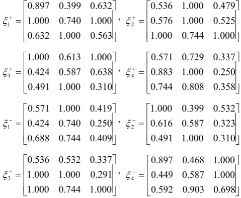
          = + 563 . 0 000 . 1 632 . 0 000 . 1 740 . 0 000 . 1 632 . 0 399 . 0 897 . 0 1 x ,           = + 000 . 1 744 . 0 000 . 1 525 . 0 000 . 1 576 . 0 479 . 0 000 . 1 536 . 0 2 x           = + 310 . 0 000 . 1 491 . 0 638 . 0 587 . 0 424 . 0 000 . 1 613 . 0 000 . 1 3 x ,           = + 358 . 0 808 . 0 744 . 0 250 . 0 000 . 1 883 . 0 337 . 0 729 . 0 571 . 0 4 x           = − 409 . 0 744 . 0 688 . 0 250 . 0 740 . 0 424 . 0 419 . 0 000 . 1 571 . 0 1 x ,           = − 310 . 0 000 . 1 491 . 0 323 . 0 587 . 0 616 . 0 532 . 0 399 . 0 000 . 1 2 x           = − 000 . 1 744 . 0 000 . 1 291 . 0 000 . 1 000 . 1 337 . 0 532 . 0 536 . 0 3 x ,           = − 698 . 0 903 . 0 592 . 0 000 . 1 587 . 0 449 . 0 000 . 1 468 . 0 897 . 0 4 x

5) Calculate the grey correlation degree of scheme matrixes

B

_k and

F

, and the grey correlation degree of

k

B

and

G

using Formula (9).

783 .

0

1+

=

γ

,

γ

₂+

=

0 .

802

,

γ

₃+

=

0 .

651

,

γ

₄+

=

0 .

688

607 .

0

1−

=

γ

,

γ

₂−

=

0 .

607

,

γ

₃−

=

0 .

789

,

709 .

0

4−

=

γ

6) Calculate the subordinate degree

u

_k of each scheme and the positive ideal scheme using Formula (12).

625 .

0

1

=

µ

,

µ

₂

=

0 .

636

,

µ

₃

=

0 .

405

,

µ

₄

=

0 .

485

This way, the final ranking result

A

₂

>

A

₁

>

A

₄

>

A

₃ could be obtained and

A

₂ is the optimal partner. This evaluation result could be used as the scientific ground by decision makers of the company. Based on the specific steps and process, it can be seen that compared with methods used in the references, the method proposed in this paper can better meet the need of practical application, and suit the real condition of problems with multi-attribute decision making better. In addition, it enjoys a higher feasibility.

5. Conclusions

(6)

decision making methods proposed in this paper is easily understandable, suitable to actual circumstances and highly feasible. Therefore, it can be widely used for further expansion and solution of similar problems with dynamic triangular fuzzy number type multi-attribute decision making.

Acknowledgements

This study was supported by the Scientific Research Fund of Hunan Provincial Education Department (No. 14C0184), by the Hunan Province Philosophy and Social Science Foundation (No. 14YBA065). It was also supported by the construct program of the key discipline in Hunan province.

REFERENCES

[1] Hu Qi-zhou, Zhang Wei-hua, Yu Li, “The research and application of interval numbers of three parameters”, Engineering Science, vol. 9, no. 3, pp. 47-51, 2007. [2] A. Banerjee, Y. Arkun, B. Ogunnaike, et al., “Estimation of

nonlinear systems using linear multiple models”, AIChE Journal, vol. 43, no. 5, pp. 1204 - 1226, May 1997.

[3] Xu Ze-shui, Da Qing-li, “New method for interval multi-attribute decision-making”, Journal of Southeast University (Natural Science Edition), vol. 33, no. 4, pp. 498-501, July 2003.

[4] Christer Carlsson, Robert Fullér, “On possibilistic mean value and variance of fuzzy numbers”, Fuzzy Sets and Systems, vol. 122, no. 2, pp. 315–326, September 2001. [5] Didier Dubois, Laurent Foulloy, Gilles Mauris, Henri Prade,

“Probability-Possibility Transformations, Triangular Fuzzy Sets, and Probabilistic Inequalities”, Reliable Computing, vol. 10, no. 4, pp. 273-297, August 2004.

[6] Chi-Bin Cheng, “Group opinion aggregationbased on a grading process: A method for constructing triangular fuzzy numbers”, Computers & Mathematics with Applications, vol. 48, no. 10, pp. 1619–1632, November 2004.

[7] Amit Kumar, Neetu, Abhinav Bansal, “A new

computational method for solving fully fuzzy linear systems of triangular fuzzy numbers”, Fuzzy Information and Engineering, vol. 4, no. 1, pp. 63-73, March 2012.

[8] Jiang Wen-qi, “Extension of VIKOR method for

multi-criteria group decision making problems with triangular fuzzy numbers”, Control and Decision, vol. 30, no. 6, pp. 1059-1064, June 2015.

[9] Huang Zhi-li, Luo Jian, “Possibility degree relation method for triangular fuzzy number-based uncertain multi-attribute decision making”, Control and Decision, vol. 30, no. 8, August 2015.

[10] A. Nagoor Gani, S. N. Mohamed Assarudeen, “A New Operation on Triangular Fuzzy Number for Solving Fuzzy Linear Programming Problem”, Applied Mathematical Sciences, vol. 6, no. 11, pp. 525 – 532, 2012.

[11] Richard Y.K. Fung, Yizeng Chen, Jiafu Tang, “Estimating the functional relationships for quality function deployment under uncertainties”, Fuzzy Sets and Systems, vol. 157, no. 1, pp. 98–120, January 2006.

[12] Su Zhi-xin, Wang Li, Xia Guo-ping, “Extended VIKOR method for dynamic multi-attribute decision making with interval numbers”, Control and Decision, vol. 25, no. 6, pp. 836-840,846, June 2010.