Is the Phillips Curve of Germany
Spurious?
Quaas, Georg and Klein, Mathias
Universität Leipzig
10 November 2010
Online at
https://mpra.ub.uni-muenchen.de/26604/
Georg Quaas / Mathias Klein
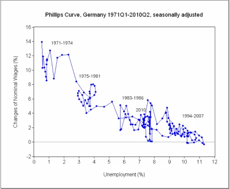
It might well be that the German Phillips Curve (Figure 1) and the corresponding
regressions (Table 1) are spurious. With “spurious” we mean a correlation, a partial
correlation or a regression equation between two variables A and B, for instance
between the change of the wage rate (A) und the unemployment rate (B), that does
not indicate a causal relationship between A (the effect) and B (the cause) but is
produced by another variable (i.e., by an underlying common cause (C), for instance
by a country’s real economic activity). This scepticism about the causal essence of
correlations and regressions can be extended to almost all important economic
relationships, which are formulated by a stochastic equation and estimated by
econometric methods, such as the well-known consumption function. The standard
interpretation of this equation is that a one-unit change of disposable income causes
a change of the amount of consumption equal to the parameter value of the marginal
propensity to consume. This cannot only be regarded with sceptical distance, but is
theoretically inverted by the Marxian interpretation that labour power’s consumption
cost causes the amount of disposable income to be an indicator of its value on the
labour market. Of course, the whole relation is controlled by a country’s economic
activity – probably a common cause, not of the consumption function only, but also of
the production function and of almost all other important econometric equations.
Nevertheless, this scepticism has had almost no effect on the development of
economic theory, like most of the critiques in the last fifty years testify (Dobusch,
Kapeller 2009).
This overall scepticism can be very productive when serving as a driving force in the
search for a common cause of a special relationship. But as long as nothing has
been found that serves as a reason for classifying a correlation as spurious, the
hypothesis that the correlation or regression is indicating a causal relationship can be
egitimized by the widely-shared Critical Rationalism as well as other schools of the
The German Phillips Curve
Quaas and Klein (2010) estimated in retro-respect several regressions that have
been of historical importance as far as they influenced the development and
consequently the shape of the modern macroeconomic theory on the price- and
wage-setting process. They used data of the German economy from 1950 to 2004
(old system of national accounts), and from 1970 to 2009 (new system of national
accounts). The common feature of all tested regressions was a very stable
relationship between the wage rate changes on the one hand and the unemployment
rate on the other, which was the original finding of Phillips (1958).
Phillips’ and especially Lipsey’s (1960) core theory that unemployment causes the
wage rate to change cannot be refuted by the application of the argument that a
nominal variable is not able to influence a real one (Phelps 1967), because the
assertion here is that a real variable influences a nominal one. Moreover, Phillips’
core assertion is part of the modern theory on wage setting as far as unemployment
still plays a crucial role in the wage-setting process.
Nevertheless, very few people are adherents to old Phillips’ finding. Theoretical
development has gone different ways, generalizing the experiences of stagflation and
hyperinflation in certain periods of time and in certain countries. Meanwhile, a
broader record of data is available, and those experiences might appear as statistical
outliers. In some aspects, “the intellectual framework for analysing the inflationary
process […] has come full circle and the Phillips curve is once again central in this
framework” (Gruen, Pagan, Thompson 1999, 253), at least for some of us. Accepting
that there is no trade-off between inflation and unemployment in the long run does
not affect Phillips’ original findings. In addition, it is a matter of fact that the data of the
German economy can be displayed in a way that is very similar to the statistical
Figure 1: Germany’s Phillips Curve, Unification data smoothed.
Statistical evidence is one thing, the theoretical interpretation another. We do not
intend to present a new theory to explain the relationship between wage rate
changes and unemployment. There are many approaches and explanations that can
be found in the theoretical debate about the determinants of wages and prices
(Eckstein, Wilson 1962; Kuh 1967; Streit 1972; Galí 2010). At the moment, we are
concerned with two reproaches to our study (Quaas, Klein 2010) presented at the
12th INFER Annual Conference 2010, which took place on 3-5 September at the
University of Muenster (Westphalia, Germany).
(i) It is likely that there is a high degree of multicollinearity among the explaining
variables, in addition to the reported high degree of autocorrelation in the error term.
parameter estimations as too optimistic. As a consequence, the results should not be
theoretically interpreted.
(ii) The wage rate changes are likely of another type of time series compared to the
unemployment rate with respect to stationarity. Therefore, the regression by which
Quaas and Klein have explained clusters and loops of the German Phillips Curve
was probably spurious, simply because the equation might be not consistent
(Granger 1981).
Are wage rate changes and unemployment rates co-integrated?
If wage rate changes and the unemployment rate are not co-integrated, serious
doubts can be cast on the causal interpretation of the Phillips Curve, especially on
the regression explaining wage rate changes by the help of the unemployment rate
(among other factors). As a matter of fact, the Augmented Dickey Fuller-test indicates
stationarity for the wage rate changes and non-stationarity for the unemployment rate
(Table 1). This fact and the high rate of autocorrelation and multicollinearity seem to
be very good reasons to doubt the results reported by Quaas and Klein (2010). This
is a scepticism that could also be directed against many regression equations that
are applied in many forecasting models of a country’s economy. Nevertheless, the
argument should be taken seriously.
In our view, the main point of the Phillips Curve is the hypothesis that there is a linear
or curve linear inverse relationship between the changes of the wage rate and the
unemployment rate – in the long run. If this is the case, both variables are necessarily
different in nature with respect to stationarity. When unemployment rates are rising,
the changes of the wage rate become smaller. By and large, this was the case in
Germany until recently, but the picture of data points makes a judgement difficult
(Figure 1).
The following steps are undertaken to create a much clearer picture of the German
Phillips Curve.
(i) We eliminated the effects of the German unification from the data by replacing the
wage rate changes of 1990 by a moving average between 1989 (the old, smaller
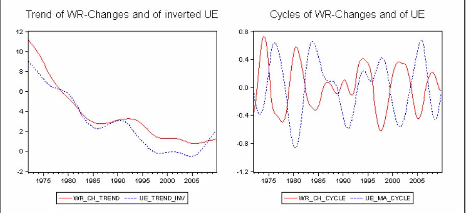
(ii) We separated the long-term tendency from the cyclical component of the relevant
time series by the help of the HP-filter.
(iii) We regressed the long-term tendency separately from the cyclical component to
see the different paths by which unemployment (UE) influences the change of the
wage rate (WR_CH).
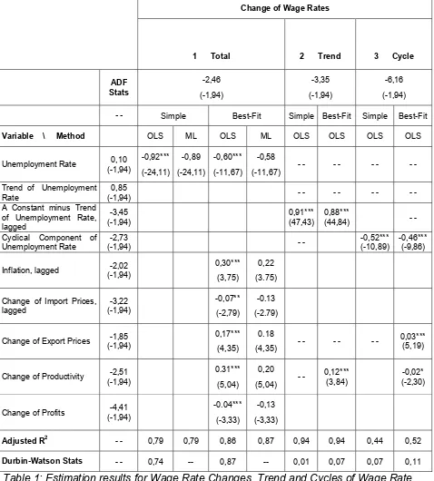
[image:6.595.71.528.277.486.2]The different curves are presented in Figure 2 and the results are reported in Table 1.
Figure 2: Trend and Cycles of Wage Rate Changes (WR_CH) and of Unemployment Rate (UE).
It turns out that the wage rate changes, and the inverse of the unemployment rate
(taken in a simplified linear version) are both stationary and therefore co-integrated.
In the long run, the lowering of wage-rate enhancements (changes) can be
Change of Wage Rates
1 Total 2 Trend 3 Cycle
ADF Stats -2,46 (-1,94) -3,35 (-1,94) -6,16 (-1,94)
- - Simple Best-Fit Simple Best-Fit Simple Best-Fit
Variable \ Method OLS ML OLS ML OLS OLS OLS OLS
Unemployment Rate 0,10
(-1,94) -0,92*** (-24,11) -0,89 (-24,11) -0,60*** (-11,67) -0,58
(-11,67) - - - - - - - -
Trend of Unemployment Rate
0,85
(-1,94) - - - - - - - -
A Constant minus Trend of Unemployment Rate, lagged -3,45 (-1,94) 0,91*** (47,43) 0,88***
(44,84) - -
Cyclical Component of Unemployment Rate
-2,73
(-1,94) - -
-0,52*** (-10,89)
-0,46*** (-9,86)
Inflation, lagged -2,02
(-1,94)
0,30***
(3,75)
0,22
(3.75)
Change of Import Prices, lagged -3,22 (-1,94) -0,07** (-2,79) -0.13 (-2.79)
Change of Export Prices -1,85
(-1,94)
0,17***
(4,35)
0.18
(4,35) - - - - - -
0,03*** (5,19)
Change of Productivity -2,51
(-1,94)
0.31***
(5,04)
0,20
(5,04) - -
0,12*** (3,84)
-0,02* (-2,30)
Change of Profits -4,41
(-1,94)
-0.04***
(-3,33)
-0,13
(-3,33)
Adjusted R2 - - 0,79 0,79 0,86 0,87 0,94 0,94 0,44 0,52
[image:7.595.69.547.87.617.2]Durbin-Watson Stats - - 0,74 -- 0,87 -- 0,01 0,07 0,07 0,11
Table 1: Estimation results for Wage Rate Changes, Trend and Cycles of Wage Rate Changes, Maximum-Likelihood estimates are standardized.
It could be argued that any falling (or rising) time series should also be capable of
explaining the falling series of wage rate changes. Therefore, we put all theoretically
relevant candidates of time series with a similar trend in the regression. It turned out
that only the long-run tendency of the inflation rate is capable of replacing the
because inflation has been considered a proxy of wage rate changes long before,
namely since Samuelson and Solow (1960).
Relevant determinants of wage rate changes
A second result consists in another stable inverse (asymmetric) relationship between
wage rate changes and the unemployment rate on the level of cyclical components of
both time series. There is an exception of some years around the German unification,
which does not fit into this scheme. Whereas in the regression of the long-term
tendency, time lags can be introduced that correspond to the hypothesised causal
order; time lags play almost no role in the explanation of the cyclical component.
Quaas and Klein (2010) reported a best-fit regression that was capable of explaining
clusters and loops of the German Phillips Curve. In Table 1 is reported which of the
explaining variables plays a significant role on the level of the long-term tendency
and on the level of the cyclical component. There is a short-term residuum (after
subtracting the long-term tendency and the cyclical component) that cannot be
explained by any of those variables. Interestingly, exactly this is the domain – the
short run – where others hypothesise a relationship of the kind Phillips has proposed.
In the best-fit regression, the single variable with the most (negative) influence is the
unemployment rate. Although we include five other variables, the unemployment rate
has kept its significant influence. This result could be an indication for a stable
long-run relationship between the unemployment rate and the changes of the nominal
wages. The estimation results of the trend and the cyclical component confirm this
observation, even though the cyclical component is not as well explained as the trend
component. But this is in line with Phillips’ discovery of a long-term relationship.
Besides the unemployment rate, the rate of change of labour productivity seems to
be a further important variable for the wage-setting process. This variable keeps its
significance in the equation of the cyclical and the trend component, while others lose
their relevance (for example the inflation rate).
In economic literature, there is a broad consensus that money wages are affected by
causes an increase of wages of about 0.30 about one year later. But inflation does
not play a role in the determination of the trend or the cyclical component of the rate
of change of wage rates.
A variable that is important not only for wage changes in total but also for its cyclical
component is the change of export prices. It reflects the special conditions of an open
economy like the German one. The positive sign sounds plausible with the following
background: A short-term change in export prices does not reduce immediately the
quantity of exports, but enhances the revenue. This also seems to be profitable for
employees.
We also tested the influence of import prices, or more precisely, a one year lag of it.
Because import prices have an influence on living cost, this information is already
included in the inflation index, the interpretation of this channel is as follows: Higher
import prices mean higher production costs for firms, and this reduces the leverage
for higher wages. But the import prices have no significant influence on the trend or
cyclical regression equations.
The same is true for the influence of profit changes on wages. Profits have a
significant negative influence on wage changes in total, but this does not hold for the
trend or the cyclical component.
In summary, the two variables that are significant in the explanation of the trend
component of the wage changes are the (inverse of the) unemployment rate and the
rate of change of productivity. For the cyclical component, it is the unemployment
rate, the change of productivity and the rate of change of the export prices that are
statistically significant.
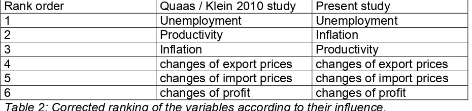
In Table 2, we put the variables in an order according to the standardized parameter
values they received in the estimation of the best-fit equation. For instance, the single
variable with the highest influence after unemployment was productivity.
As can be seen in Table 2, there are only minor changes of the estimates based on
standardised variables, and consequently only minor changes on the rank order of
Rank order Quaas / Klein 2010 study Present study
1 Unemployment Unemployment
2 Productivity Inflation
3 Inflation Productivity
[image:10.595.67.532.93.203.2]4 changes of export prices changes of export prices 5 changes of import prices changes of import prices 6 changes of profit changes of profit
Table 2: Corrected ranking of the variables according to their influence.
Conclusion
The problem of multicollinearity is reduced (Intriligator 1978, 267-268) when fewer
variables are used in a regression. This reduction is necessary when trend and
cyclical component of the Phillips Curve are explained separately. It turns out that
this does not affect the decisive role the unemployment rate plays in the explanation
of wage rate changes. Admittedly, autocorrelation is very high in the regressions on
the level of the trend and of the cyclical component. Therefore, t-statistics may be
misleading. As we said in the introduction, we cannot exclude that the reported best
fit regression is spurious, but the allegedly missing co-integration of wage rate
References
Dobusch, L. / Kapeller, J. (2009), Why is Economics not an Evolutionary Science?
New Answers to Veblen’s Old Question, Journal of Economic Issues 43, 867-898.
Eckstein, O. / Wilson, T. A. (1962), The Determination of Money Wages in American
Industry, Quarterly Journal of Economics 76, 379-414.
Galí, J. (2010), The Return of the Wage Phillips Curve.
Granger, C. W. J. (1981), Some Properties of Time Series Data and their USE in
Econometric Model Specification, Journal of Econometrics 16, 121-130.
Gruen, D. / Pagan, A. / Thompson, C. (1999), The Phillips curve in Australia, Journal
of Monetary Economics 44, 223-258.
Intriligator, M., Econometric Models, Techniques and Applications. Amsterdam 1978.
Kuh, E. (1967), A Productivity Theory of Wage Levels – An Alternative to the Phillips
Curve, Review of Economic Studies 34, 333-360.
Lipsey , R. G. (1960), The Relation between Unemployment and the Rate of Change
of Money Wage Rates in the United Kingdom, 1862-1957: A Further Analysis,
Economica 27, 1-31.
Outhwaite, W., New Philosophies of Social Science. London 1987.
Phelps, E. S. (1967), Expectations of Inflation and Optimal Unemployment over Time,
Economica 34, 254-281.
Phillips, A. W. (1958), The Relation between Unemployment and the Rate of Change
Quaas, G. / Klein, M. (2010), Clusters and Loops of the German Phillips Curve.
MPRA-Paper #23094, published at 06-06-2010,
http://mpra.ub.uni-muenchen.de/23094/
Samuelson, P. A. / Solow, R. M. (1960), Analytical Aspects of Anti-Inflation Policy,
American Economic Review 50, 177-194.
Streit, M. E. (1972), The Phillips curve: Fact or fancy? — The example of West
Germany, Review of World Economics 108, 607-633.
Data Sources
StBA, Volkswirtschaftliche Gesamtrechnung, Fachserie 18, Reihe S.21, Revidierte
Ergebnisse 1970-2004, March 2005.
StBA, Volkswirtschaftliche Gesamtrechnungen, Fachserie 18, Reihe 1.5,
Inlandsproduktsberechnung, Lange Reihen ab 1970, Februar 2010.
StBA, Volkswirtschaftliche Gesamtrechnungen, Fachserie 18, Reihe 1.2,
Inlandsproduktsberechnung, Vierteljahresergebnisse, Zusatztabellen, Tabelle
Unverketteten Volumenangaben, Mai 2010.
Agentur für Arbeit, Aktuelle Daten - Arbeitslose nach Rechtskreisen.
http://www.pub.arbeitsamt.de/hst/services/statistik/detail/a.html
Agentur für Arbeit, Zeitreihen – Arbeitslosigkeit in Deutschland seit 1950.
http://www.pub.arbeitsamt.de/hst/services/statistik/detail/z.html
Definitions, Indicators, and Data
www.forschungsseminar.de/phillips.htm