Munich Personal RePEc Archive
Political ideology as a source of business
cycles
marina, azzimonti
university of texas -austin
June 2010
Online at
https://mpra.ub.uni-muenchen.de/25937/
Political ideology as a source of business cycles
∗Marina Azzimonti†
This version: June 2010
Abstract
When the government must decide not only on broad public-policy programs but also on the provision of group-specific public goods, dynamic strategic inefficiencies arise. The struggle between opposing groups–that disagree on the composition of expenditures and compete for office–results in governments being endogenously short-sighted: systematic under-investment in infrastructure and overspending on public goods arises, as resources are more valuable when in power. This distorts allocations even under lump-sum taxation. Ideological biases create asymmetries in the group’s relative political power generating endogenous economic cycles in an otherwise deterministic environment. Volatility is non-monotonic in the size of the bias and is an additional source of inefficiency.
JEL Classification: E61, E62, H11, H29, H41, O23
Keywords: Public Investment, Commitment, Probabilistic Voting, Markov Equilibrium, Po-litical Cycles, Time Consistency.
∗An earlier version of this paper circulated under the title ‘On the dynamic inefficiency of governments’. I would
like to thank Steve Coate, Per Krusell, Fernando Leiva Bertran, Lance Lochner, Leo Martinez, Antonio Merlo, Victor Rios-Rull, Pierre Sarte and Andrzej Skrzypacz as well as participants of the SED Meeting, the Midwest Macroeconomics Meetings, the Public Economic Theory Conference and the Prague-Budapest Spring Workshop in Macroeoconomic Theory. I would also like to thank attendants to the department seminar series at the FRB of Richmond and the universities of Rochester, Iowa, and British Columbia for helpful comments. Part of this work was developed while visiting the IIES at Stockholm University and the University of Pennsylvania. All errors are mine.
1
Introduction
Public policy and institutions are found to be relevant factors in explaining the large differences in
income per-capita across countries.1 However, policies that enhance growth and promote
develop-ment are not always chosen by the governdevelop-ment (especially in under-developed economies). Why? A group of explanations attributes it to the instability that results from major political upheaval
and coups d’etat.2 It turns out that even democratic countries, where changes in government follow
a stable election process, exhibit large disparities in income and implemented policies. Several au-thors suggest that this could be the result of failures or frictions in the decision-making process of
the public sector.3 A basic point is that policymakers can engage in rent-seeking activities and may
choose inefficient policies in order to increase their probability of re-election so as to get continued
access to these office rents.4 However, one does not need to take such a cynical view of governments.
Even governments that are not “intrinsically bad” can, due to the democratic process itself—where reelection is never certain—and the resulting natural lack of commitment, generate bad outcomes. This is the idea pursued in the present paper.
I present a theoretical model where the struggle between groups with different views that
alter-nate in power results in governments being endogenouslyshort-sighted—at least more so than the
groups they represent. As a consequence, they tend to overspend and underinvest, reducing output and private consumption. The party in power tries to tie the hands of its successor by strategically manipulating public investment. Political uncertainty, together with the assumption of a funda-mental lack of commitment, creates incentives to reduce the amount of public capital available for the next policymaker as a way to restrict his level of spending. I show that the dynamic inefficiency generated by the politician’s short-sightedness is mitigated by the degree of political stability. In addition, asymmetries in the groups’ relative political power—which result from ideological biases
in the population—generate endogenous economic cycles. Macroeconomic variables fluctuate in
equilibrium, even in the absence of productivity shocks. Analyzing the implications of this second source of inefficiency will be the objective of this paper.
In this economy, the role of the government is to provide public goods and invest in productive public capital, which are financed through lump-sum taxation. There are two groups in the economy that disagree over the composition of spending on public goods but not over its aggregate size or over the level of infrastructure investment. Groups are represented by parties which alternate in power via a democratic process, and election outcomes are uncertain. The degree of political stability (i.e. frequency of turnover) is determined in a voting equilibrium. Agents are forward looking and vote for the party that yields them higher expected utility. I consider a situation where voter’s ideological biases towards one the groups yields its candidates a political advantage over those from the other group, which leads to an asymmetric equilibrium. There is no commitment technology, so promises made during the campaign are non-binding. I characterize time-consistent outcomes as Markov-perfect equilibria. I first derive the incumbent’s optimality condition for a general case and characterize the determinants of political turnover in the equilibrium of a voting model. Thus, the degree of political uncertainty is jointly determined with public policy, so it depends on the primitives that shape it (i.e., on the intensity of ideology, on agent’s preferences, and on technology). I then find an analytical solution under specific functional assumptions in
1For example, Acemoglu, Johnson, Robinson (2001) study the relationship between property rights and different
degrees of development.
2Barro (1996) and Easterly and Rebelo (1993) provide evidence that coups reduce growth.
3See Persson and Tabellini (1999) for an excellent review of the literature.
4An analysis of the earlier models in this literature (e.g. Barro, Nordhaus, and Ferejohn) can be found in Drazen
order to derive testable implications from the theory. Finally, I present some empirical evidence supporting the model predictions.
I find that the group that has an advantage in the political dimension (i.e., its candidates are more ‘popular’) wins the elections more often and spends a lower share of output on public consumption, while investing a larger share than its counterpart. The political uncertainty is propagated into the economy and endogenous economic cycles are generated, even though there is no source of uncertainty other than the identity of the policymaker. This decreases welfare relative to the first best not only because it reinforces the dynamic inefficiency (investment is too low), but also because it introduces volatility in macroeconomic variables (output, employment, and consumption). Increases in the ideological bias widen the gap between the policies chosen by the the two groups, as well as their probabilities of being elected. The size of business cycles induced by changes in the bias is non-monotonic because it is affected by changes in policy and probabilities in opposite directions. As a result, economies where the political advantage is low exhibit rapid turnover but small fluctuations in policy as the gap in investment shares is small. At the other extreme, when the biases are large so are the differences in policy, but the most popular party is in power more often and hence fluctuations are small. Volatility is largest for intermediate values of the ideological bias. Using a proxy for investment shares and ideology biases for the US during the period 1929-2006, I show that these two variables tend to comove, providing some support for the theory.
On a more methodological level, this paper provides an optimality equation faced by the gov-ernment in power that can be used to analyze the trade-offs that arise in the presence of reelection uncertainty. It reveals that there is a wedge between the marginal cost and marginal benefit of
in-vestment when compared to the benevolent planner’s solution (so allocations areinefficient). This
wedge arises from the existence of intertemporal strategic effects. On the one hand, the government wants to decrease the level of resources available to next period’s policymaker so as to restrict his level of spending. But this will cause a negative effect in the opposition’s investment level, which the incumbent may want to boost if it expects the opposition to invest too little. On the other hand, changes in policy may also modify reelection probabilities, which must be taken into account by forward-looking governments.
Existing Literature
This paper contributes to a literature that analyzes the dynamic efficiency of policy choice in representative democracies. It builds on the work by Besley and Coate (1998) and Alesina and Tabellini (1990) who present the first theories of political failure. In Alesina and Tabellini (1990) parties choose to overspend in public goods and to create an excessive level of debt when the outcome of elections is uncertain. In Besley and Coate (1998) parties fail to undertake a public investment that is potentially Pareto improving due to lack of commitment in a two-period model. Our work extends some of their insights to a dynamic infinite-horizon political economy model, particularly relevant for assessing the long-run effects of current policy.
One of the papers most closely related to this is Amador (2008) who also analyzes the inef-ficiencies generated by a common pool problem in a dynamic infinite horizon model. His basic mechanism, like the one in this paper, is based on the trade-offs described in Alesina and Tabellini (1990). Amador finds that politicians are too impatient behaving as hyperbolic consumers, which results in inefficient overspending and excessive deficit creation. In his paper the alternation of
power is exogenous, while it is determined by voting in the current paper.5 Azzimonti (2010)
endo-genizes political turnover in a similar environment where the government distorts private investment
in order to finance group specific public goods. Overspending results in equilibrium, but there is no public investment. Battaglini and Coate (2007) introduce productive public goods financed by the government. Instead of focusing on political parties, they assume that policy is decided through legislative bargaining. In their work the probability of being able to choose expenditures is exoge-nous and only depends on the number of legislators, while it is endogeexoge-nous here and depends on the level of public investment. Additionally, distortions arise due to the assumption of proportional taxation on labor income in their paper, while I assume those away by focusing on lump-sum taxes (distortions arise because public capital affects the productivity of labor here, while the two are
completely independent in their setup). 6 In addition, in these three papers parties are completely
symmetric so there are no fluctuations in macroeconomic variables induced by changes of power. The analysis of business cycles generated by ideological biases is a main contribution relative to their work.
This paper also contributes the literature on inefficiencies resulting from the government’s lack of commitment. While existing models with repeated voting find strategic interactions, most of them must rely on numerical methods to characterize the Markov-perfect equilibrium (i.e. Krusell and Rios-Rull 1999). Hassler, Mora, Storesletten, and Zilibotti (2004), on the other hand, find analytical solutions in an overlapping generations setup where policy is decided by majority voting, but assume away political uncertainty. Hassler, Storesletten, and Zilibotti (2007) find that expenditures in a consumable public good can be inefficient, but in a model where two-period lived agents vote over redistributive policy. Unlike in their work, part of the expenditures are devoted to productive investment, which allows us to analyze the effects of policy on economic development.
I also extend existing work by endogenizing the probabilities of reelection in a dynamic setup. A key assumption in this paper is that politicians are citizen candidates that do not have com-mitment to platforms. As a result, voters expect the incumbent to maximize the utility of the group he represents (disregarding the welfare of other groups). This is opposite to standard result in probabilistic voting models with commitment to platforms, where the politicians maximization problem is equivalent to that of a benevolent planner (see Sleet and Yeltekin, 2008 or Farhi and Werning, 2008). In a recent paper Battaglini (2010) considers an environment where expected ideological biases are persistent and candidates are office seekers with commitment to platforms. He finds that the political equilibrium exhibits excessive debt creation and over spending. Due to the assumption that there is no ex ante bias in favor or against any candidate, the equilibrium is symmetric. Therefore, there are no fluctuations in debt, taxes or macroeconomic variables gener-ated by switches of power (other than those resulting from productivity shocks), which is the focus of this study.
Finally, this paper is related to the literature on ‘partisan cycles’. In contrast to previous models in this literature (like Milesi-Ferreti and Spolaore, 1994, Persson and Svensson, 1989 or more recently Song, 2009), I do not need to assume exogenous differences in preferences over the size of public expenditures in order to generate fluctuations. Parties have the same ex-ante utility over the size of spending on public goods and on the level of investment. In equilibrium one party may spend more and invest less just because it loses more often as a result of an ideological disadvantage.
The organization of the paper is as follows. The model is described the Section 2 and the Markov-perfect equilibrium defined in Section 3. An analytical solution is presented in Section
analyze environments where exogenous political turnover introduces inefficiencies in debt accumulation and the level of taxation in Markov-switching models. See Lagunoff and Bai (2010) for an interesting case where the probabilities are exogenous but depend on the aggregate state of the economy.
6Besley, Ilzetzki, and Persson (2010) study the effects of exogenous political instability on fiscal capacity (a durable
4, where qualitative and quantitative implications are derived. Section 5 provides some empirical support for the theory and Section 6 concludes.
2
The basic model
2.1 Economic environment
Consider an infinite-horizon economy populated by agents that live in one of two regions, A and
B, of measure µJ = 1
2, J = {A, B}. While they have identical income and identical preferences
over private consumption, they disagree on the composition of public expenditures since public goods can be region-specific (e.g. parks, museums, environmental protection, public television, etc). Agents also differ in another dimension that is orthogonal to economic policy (religious views,
charisma of the politician, etc.). Preferences over thispolitical dimension imply derived preferences
over candidates, and will take the form of additive iid preference shocksξ (to be described in more
detail later). The instantaneous utility of agentj in region J at a particular point in time is
u(cj, nj) +v(gJ)
economic
+ ξj
political
, (1)
where u and v are increasing and concave in c and g, and u is decreasing inn, with v(0) ≡v¯,cj
denotes the consumption of private goods, nj denotes labor, and gJ is the level of discretionary
spending on local goods in regionJ. Notice that an agent living in regionAderives no utility from
the provision of a good in region B (and vice versa), so in principle there will be disagreement in
the population over the desired composition of public expenditures, but not on its size, since both types have the same marginal rate of substitution between private and public goods.
There are infinitely many competitive firms that produce a single consumption good and hire labor each period so as to maximize profits, which are distributed back to consumers who own shares
of these firms. Firms have access to a Cobb-Douglas technology: F(Kg, n) =AKgθn1−θ,wherenis
the aggregate labor supply and Kg is the stock of public capital (i.e. infrastructure, public health,
and education, the knowledge produced by the public sector’s R&D and expenditures in national defense or law enforcement). Its level is determined by government investments and acts as an externality in production. The idea behind this specification is that the better the infrastructure (roads, harbors, sewers, etc.), the more educated the population and the stronger the protection of property rights, the higher the productivity of the private sector.
The government raises revenues via lump-sum taxesτ which are chosen every period, so private
consumption is
cj =wnj+π−τ.
Taxes are used to finance the provision of consumable public goods (gAandgB) and investments
on productive public capital (IKg). The cost of producing g > 0 units of a local public goods is
given by x(g), with x(0) = 0. Assuming that there is no debt, the government must balance its
budget every period, so its budget constraint reads as:
J
x(gJ) +IKg =τ.
Assuming a depreciation rate of δ, public capital evolves according to:
where primes denote next period variables. The assumption of lump-sum taxes is made in order to highlight that inefficiencies in production may arise due to political frictions even when the government has access to non-distortionary financing instruments.
2.2 Planning solutions
Before describing the outcome under political competition (where different parties alternate in power), it is useful to characterize the optimal allocation chosen by a benevolent social planner.
The planner chooses{c, K′
g, gA, gB}so as to maximize a weighted sum of utilities, where the weight
on typeJagents isλJ(withλA+λB= 1). All individuals within groupJare treated in a symmetric
way since their political shocks are irrelevant for the determination of economic allocations. The planner’s maximization problem follows.
V∗(Kg) = max
J
µJλJ[u(c, n) +v(gJ)] +βV∗(Kg′),
subject to the resource constraint:
J
x(gJ) +c+Kg′ =F(Kg, n) + (1−δ)Kg.
As long as the planner gives a positive weight to each agent, the optimal allocation of public
good J will be such that its marginal utility is proportional to the marginal utility of private
consumption.7
u1(c, n)xg(gJ) =ζJvg(gJ), whereζJ =
λJ
JλJ
<1. (2)
By varying λJ between 0 and 1 it is possible to trace the Pareto frontier that characterizes the
optimal provision of public goods. Concavity ofvimplies that if typeAagents have a higher weight
in the social welfare function, more of their desired public good will be provided (at the expense of
type B agents).
Labor satisfies a standard first order condition where
u1(c, n)F2(Kg, n) +u2(c, n) = 0.
Finally, the planner chooses the level of public capital that equates the marginal costs in terms of foregone consumption to the discounted marginal benefits of the investment.
u1(c, n) =βu1(c′, n′)[F1(Kg′, n′) + 1−δ]. (3)
The planner’s Euler equation is completely independent of the choice of the social welfare function:
changes in λJ do not affect this margin. The results follows from assuming that both agents have
the same trade-off between private and public consumption (i.e. u and v are equal for all agents).
It is important to note that the planner is constrained to offer all households the same
con-sumption allocation (that is,cA=cB). This is imposed in order to capture the constraint faced by
the government in the political equilibrium (where parties cannot tax agents at different rates).8
7If the planner only cares about the well-being of, say, agentA, it will setgB
t = 0∀tandgtAso as to equate the
marginal rate of substitution between private and public goods to the marginal cost of providing the goodsxg(g).
8If we were to assume that λAµA = λBµB, the unconstrained social optima would coincide with the result
3
Political equilibrium
The role of the government in this economy is to provide public goods and productive public capital. Given the disagreement between groups over which public good should be provided, political parties will endogenously arise in a democratic environment. I analyze a stylized case where there are two
parties,Aand B,representing each group in the population and competing for office every period.
There will be no distinction between a ‘candidate’ and a ‘party’ (all candidates have the same preferences so there is no heterogeneity within a party).
The groups will alternate in power based on a political institution where “ideology” or other non-economic issues play a role. In particular, I use a “probabilistic-voting” setup (see Lindbeck and Weibull (1993)) in order to provide micro-foundations for political turnover: the probability of being in power next period is going to be endogenously determined via an electoral process. A key
departure from the traditional probabilistic voting model is thatparties do not have commitment
to platforms, so announcement made during the political campaign will not be credible unless they are ex-post efficient (that is, once the party takes power). The elected party decides on the level of taxes and the allocation of government resources between spending and investment. Its objective
is to maximize the utility of its own type. 9
Timing
Each period will be divided into three stages: the Taxation Stage, the Production Stage and the Election Stage.
At the Taxation Stage, the incumbent choosesτ, gA, gBandK′
gknowing the state of the economy
(Kg) and the distribution of political shocks but not their realized values. Hence, policy is chosen
under uncertainty. The probability of winning the election can be calculated by forecasting how agents vote given different realizations of the shock.
At the Production Stage agents choose labor supply and levels of consumption taking policy as given, but under uncertainty about the identity of future policymakers. Firms hire labor and distribute profits, and the government implements the policy chosen by the party in power.
After production, consumption, and investment take place,ξ′ is realized. At the Election Stage,
agents vote for the party that gives them higher expected lifetime utility. They need to forecast how the winner of the election chooses policy. The assumptions of rationality and perfect foresight imply that agents’ predictions are correct in equilibrium.
3.1 Markov-perfect equilibrium
There is no commitment technology, so promises made by any party before elections are not credible unless they are ex-post efficient. The party in power plays a game against the opposition taking their policy as given. Alternative realizations of history (defined by the sequence of policies up
to time t) may result in different current policies. In principle, this dynamic game allows for
multiple subgame-perfect equilibria that can be constructed using reputation mechanisms. I will rule out such mechanisms and focus instead on Markov perfect equilibrium (MPE), defined as a set of strategies that depend only on the current—payoff relevant—state of the economy. Given the sequence of events and the separability assumption between the economic and the political dimensions, the only payoff-relevant state variable is the stock of public capital. In a Markov-perfect equilibrium, policy rules and voting decisions are functions of this state. Since there is no
9In that sense this is a partisan model, see Drazen (2000) or Persson and Tabellini (2000) for a description of
commitment and no retrospective voting, the values of gA and gB chosen by the incumbent are irrelevant in the voting decision. So is the history of ideology shocks, since there is no persistence. The equilibrium objects that we are interested in are policy functions, allocations, winning probabilities, and value functions. There are three policy functions: the investment rule of incum-benti,hi(Kg), and expenditures in each region-specific goodgAi (Kg) andgiB(Kg). Agentj’s labor
supply nij(Kg) and consumption cij(Kg) under incumbent i’s policies summarize the allocations
(firms decisions as well as aggregate consumption and labor supply can be trivially determined from
these functions). The probabilities will be denoted bypi(Kg).The value function—net of political
shocks—of agentjwhen his group is in power will be denoted byVj(Kg) and when his group is out
of power by Wj(Kg). The characterization of the MPE follows, starting from the last stage (the
Election stage) to make the exposition clearer.
Election Stage
At this stage, agents must decide which party to vote for. The utility derived from political
factors, ξj, has two components: an individual ideology bias (denoted by ϕjJ) and an overall
popularity bias (ψ). In particular,
ξi=ψ+ϕjJ Ii,
whereIis an indicator function such thatIB= 1 andIA= 0, since the individual specific parameter
ϕjJ measures voter j ’s ideological bias towards the candidate from partyB.I will follow Persson
and Tabellini (2000) by assuming that the distribution ofϕjJ is uniform and group-specific,
ϕjJ ∽
− 1
2φJ,
1 2φJ
, withJ =A, B.
These shocks are iid over time, hence ‘candidate specific.’ Each period, a given party presents a
candidate and voters form expectations about the candidate’s position on certain moral, ethnic or religious issues, orthogonal to the provision of public goods. Examples are attitudes towards crime (gun control or capital punishment), drugs (i.e. whether to legalize the use of marijuana), immigration policies, pro-life or pro-choice positions, same sex marriage, etc. A value of zero indicates neutrality in terms of the ideological bias, so agents only care about the economic policy,
while a positive value indicates that agent j prefers party B over A. Since ϕjJ can take positive
or negative values, there are members in each group that are biased towards both candidates. Therefore, individuals belonging to the same group may vote differently.
The parameter ψ represents a general bias towards partyB at each point in time. It measures
the average relative popularity of candidates from that party relative to those from partyA. While
the realization ofϕjJ is individual-specific, the value of ψis the same for all agents. 10 It captures
candidates’ personal characteristics such as honesty, leadership, integrity, charisma, trustworthiness,
etc. Candidates with higher values ofψ are preferable by all agents.
The popularity shock isiidover time and can also take positive or negative values. It is distributed
according to:
ψ∽
−1
2+η,
1
2+η
.
A positive value for η (the expected value of ψ) implies that candidates from party B have an
average popularity advantage over those from the opposition. On the other hand, η = 0 implies
10Political scientists refer to this parameter asvalence, referring to “issues on which parties or leaders are
that parties are symmetric, in the sense that their candidates are expected to be equally popular or charismatic.
Finally, agents are assumed to have perfect information about the candidates, so there are no informational asymmetries in this model. At the election stage, voters compare their lifetime utility
under the alternative parties. The maximization problem of voter j in groupA is given by
maxVA(Kg′), WA(Kg′) +ψ′+ϕjA′
,
where VA(Kg′) denotes the welfare of this agent if a candidate representing his group wins the
elections, whileWA(Kg′) is the value of his utility if the candidate representing groupB is elected.
The maximization problem of an agent in groupB is analogously defined.
Determination of probabilities
Let’s turn now to the intermediate stage between taxation and voting, where the shocks have not yet been realized.
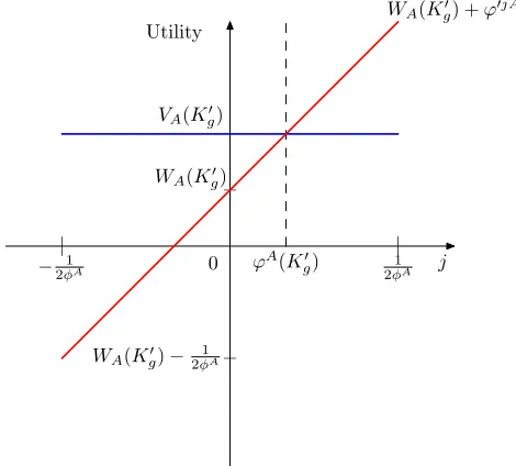
Individualj ∈A votes for B whenever the shocks are such that
VA(Kg′)< WA(Kg′) +ψ′+ϕjA′.
We can identify theswing voter in groupA as the voter whose value ofϕjA′ makes him indifferent
between the two parties
ϕA(Kg′) =VA(Kg′)−WA(Kg′)−ψ′.
Figure 1 illustrates this point (assumingψ= 0 for simplicity). The swing voter is found where the
two solid lines intersect. All voters in groupA with ϕjA′ > ϕA(K′
g) also prefer party B as can be
seen in the graph.
The same type of analysis can be performed for agents in groupB,to determine the swing voter
in that group. The value ofϕJ depends on the difference in utilities of having groupAvs group B
being in office and on the realization of the popularity shock.
Given the assumptions about the distributions of ϕjA and ϕjB the share of votes for party B
is:
πB=
J
µJPϕjJ′> ϕJ(Kg′)
= 1
2 −
J
µJφJϕJ(Kg′).
Under majority voting, partyB wins if it can obtain more than half of the electorate; that is, if
πB > 12.This occurs whenever its relative popularity is high enough. There exists a threshold for
ψ, denoted by ψ∗(K′
g) such that B wins for any realization ψ > ψ∗(Kg′). After performing some
algebra using the expression above, we find that
ψ∗(Kg′) = 1 φ
µAφAVA(Kg′)−WA(Kg′)
+µBφBWB(Kg′)−VB(Kg′) , (4)
where φ=µAφA+µBφB.
The threshold is given by a weighted sum of the differences in the utility of the swing voter under each party. The weights depend on the dispersion in the ideology shocks and on the amount
of supporters that each party has. The higher the heterogeneity within a constituency (φJ), the
individuals belonging to type J, the stronger the group in the determination of the probability. Finally, note that the threshold depends on the level of public capital, though it is not clear in
which direction. In principle, this level could increase or decrease withK′
g.
Since ϕJ(K′
g) depends on the realized value ofψ,ex-ante the share of votes for partyB (πB) is
a random variable. B’s probability of winning the election is given by:
pB(Kg′) = P
πB>
1 2
= P(ψ′ > ψ∗(Kg′)),
which is equivalent to:
pB(Kg′) =
1
2 +
η−ψ∗(Kg′). (5)
A’s probability of winning the next election is just pA(Kg′) = 1−pB(Kg′).
Recall that η represents the popularity advantage of candidates from party B over those from
party A.So in principle,B’s probability increases with η.
The current level of consumption in private and public capital does not affect the voting decision (i.e. no retrospective voting). Voters do not ‘punish’ politicians/parties for their past behavior but decide instead in terms of future expected policy choices.
Production Stage
At this stage firms decide how much labor to hire given wages, and distribute profits back in the form of dividends to agents, who own shares of these firms. Agents choose consumption and leisure, taking wages and government policy (public spending and investment) as given. A
competitive equilibrium given policy is defined below, where we omit the stock of public capitalKg
from all functions to simplify the notation.
Definition 1: A competitive equilibrium given government policy Υ = {gA, gB, K′
g} is a set of
allocations, {cj(Υ), nj(Υ),Π(Υ)}, prices w(Υ), and taxes τ(Υ) such that:
(i). Agents maximize utility subject to their budget constraint. Agentj’s labor supply satisfies
u1(cj(Υ), nj(Υ))w(Υ) +u2(cj(Υ), nj(Υ)) = 0,
where
cj(Υ) =w(Υ)nj(Υ) + Π(Υ)−τ(Υ).
(ii). Firms maximize profits, sow(Υ) =F2(Kg, n(Υ)) and Π(Υ) =F(Kg, n(Υ))−w(Υ)n(Υ).
(iii). Markets clear n(Υ) =JµJn
j(KgΥ).
(iv). The government budget constraint is satisfied.
τ(Υ) =
J
x(gJ) +Kg′ −(1−δ)Kg.
The static nature of firms’ and workers’ economic decisions simplifies the characterization of the competitive equilibrium to a great extent. Moreover, from condition (i) we can see that agents’
decisions are independent of their typej, which results from the additive separability of the political
shock. Hence, there is aggregation and we can think of the economic dimension as being
firm’s optimal decisions and the government budget constraint into the agent’s budget constraint we obtain consumption as a function of policy,
c(Υ) =F(Kg, n(Υ)) + (1−δ)Kg−
J
x(gJ)−Kg′, (6)
with labor as satisfying
u1(c(Υ), n(Υ))F2(Kg, n(Υ)) +u2(c(Υ), n(Υ)) = 0. (7)
The last two expressions allow us to write agent’s indirect utility, since they summarize the private sector reaction to alternative policies.
Taxation Stage
At this stage, the incumbent must decide on the optimal policy knowing that he will be replaced
by a different policymaker with some probability. Suppose that B is the elected party. Given the
stock of public capital Kg, his objective function today is:
max
gA,gB,K′
g≥0
u(c, n) +v(gB) +ξj+β{pB(Kg′)VB(Kg′) +pA(Kg′)WB(Kg′) +EB(ξ′j;Kg′)} (8)
where consumption and labor satisfy equations (6) and (7), WB denotes the utility of a type
B agent when his party is out of power. EB(ξj′, Kg′) represents the expected value of tomorrow’s
political shock conditional on B winning the next election (recall that this shock is a relative bias
towards a candidate form party B),
EB(ξj′;Kg′) =
1 2+η
ψ∗(K′
g) z∂z,
which can be shown to be equal to
EB(ξj′;Kg′) =pB(Kg′)
1 2pA(K
′
g) +η
.
By changing the stock of public capital the incumbent affects not only the economic dimension
but also his probability of winning and the expected value of political shocks. 11
Since gA and gB only affect today’s utility, tomorrow’s decisions are independent of the
com-position of expenditures. If party i is in power, it will choose gJ
i = 0, for J = i, which further
simplifies the problem. Slightly abusing notation, we usegi(Kg) to denote the equilibrium amount
spent by incumbenti on the local public goodi. The description of the problem is completed by
defining the functions VB(Kg) and WB(Kg):
VB(Kg) =u(cB(Kg), nB(Kg)) +v(gB(Kg))+ (9)
β{pB(hB(Kg))VB(hB(Kg)) +pA(hB(Kg))WB(hB(Kg)) +EB(ξj′;hB(Kg))}
and
WB(Kg) =u(cA(Kg), nA(Kg)) + (10)
11Other papers in the literature usually ignore political shocks because they study two period models, once the
shock has been realized. Since ξ is additive, focusing on net-of-shock welfare is without loss of generality. In this
β{pB(hA(Kg))VB(hA(Kg)) +pA(hA(Kg))WB(hA(Kg)) +EB(ξj′;hA(Kg))},
where Υi(Kg) ={giA(Kg), gBi (Kg), hi(Kg)} denotes the equilibrium policy functions chosen by
incumbent type i, and where ci(Kg) = c(Υi(Kg)) and ni(Kg) = n(Υi(Kg)) are the competitive
equilibrium values of consumption and labor under the political equilibrium policies.
The choice of expenditures is a static one, affecting only the intra-temporal margin. At the
optimum, the government chooses g so that the marginal cost of providing the good in terms of
consumption equals its marginal benefit:
u1(cB(Kg), nB(Kg))xg(g) =vg(g). (11)
We can see that government spending in the MPE is sub-optimal from the standpoint of an utili-tarian social planner by comparing eq. (2) to the equality above. This is the case for two reasons. First, the group out of power gets no provision of their preferred good. Second, there is over-spending in the sense that the marginal rate of private consumption is too low when compared to
that of the utilitarian optimum. Even the group in power would prefer a lower level of g if the
difference was invested in productive capital and subsequently used in the provision of its preferred good instead.
The investment decision affects theinter-temporal margin; the costs of increasing public capital
are paid today while the benefits are received in the future. The government chooses K′
g so that
the marginal cost in terms of foregone consumption equals expected marginal benefits:
u1(cB(Kg), nB(Kg)) =β{pB(Kg′)VB1(Kg′) +pA(Kg′)WB1(Kg′)
+pB1(Kg′)
VB(Kg′)−WB(Kg′)
+EB2(ξj′;Kg′)},
wherepB1(Kg′) =
∂pB(Kg′)
∂K′
g , and we use the fact thatpA= 1−pB.
Even though parties represent their constituencies and have no derived value of being in office, they will try to manipulate the probability of being re-elected (which allows them to implement the desired policy in the future).
As in the planner’s first-order condition, the cost of an extra unit of investment in public capital
is given by a reduction in current utility via a decrease in consumption −u1(c, n). The benefits,
on the other hand, now depend on the identity of the party that wins the next election. When K′
g
increases, expected future utility rises from the expansion of resources. Type B agents enjoy an
increase of VB1(Kg) =
∂VB(Kg′)
∂K′
g utils if they win the next election (which occurs with probability
pB) and WB1(Kg) =
∂WB(Kg′)
∂K′
g otherwise (which occurs with probability pA= 1−pB). Given that
the identity of the decision-maker changes over time, the envelope theorem doesn’t hold in this environment, so the traditional Euler equation will not be satisfied. A change in investment today also modifies the problem faced by voters, which in turn affects the probability of being in power next period. A rational incumbent realizes this and thus takes into account the effect of expanding K′
gon its likelihood of winning. It is reasonable to expect thatVB(Kg′)> WB(Kg′),a group is better
off while in power. However, the sign of pB1(Kg′) is, in principle, ambiguous. On the one hand,
we expect that the richer the economy, the lower the political turnover (i.e. the probability of an incumbent losing the election decreases, so that the same party tends to stay in power longer). This would imply that by increasing the level of productive capital, the incumbent can tilt the election in
its favor, which creates an extra indirect benefit of having moreK′
g. On the other hand, ifpB1(Kg′)
only current consumption but also future utility via the indirect effect of reducing the probability of winning the next election.
Politico-economic equilibrium
We can now define a political equilibrium that takes into account agent’s voting decisions.
Definition A Markov-perfect equilibrium with endogenous political turnover is a set of value and policy functions such that:
i. Given the re-election probabilities and CE allocations and prices, the functions hi(Kg),
gBi (Kg), giA(Kg), Vi(Kg), and Wi(Kg) solve incumbent i′s maximization problem, given by
equa-tions (8), (9), and (10).
ii. Given the re-election probabilities and government policy, the functions ci(Kg) and ni(Kg)
satisfy equations (6) and (7).
iii. Given the optimal rules of the government and CE allocations and prices, pB(Kg) solves
eq. (5) and pA(Kg) = 1−pB(Kg).
The definition just imposes consistency between private agents and government’s decisions at every stage (taxation, production, and election).
3.2 Differentiable Markov Perfect Equilibrium (DMPE)
In order to further characterize the trade-offs faced by an incumbent when choosing investment,
I will focus on differentiable policy functions. Klein, Krusell, and Rios-Rull (2008) made this
assumption (in a different context) arguing that there could be in principle an infinitely large number of Markov equilibria. By assuming differentiability, the problem delivers a solution that is the limit to the finite horizon problem. Moreover, it allows us to derive the government optimality
condition: 12
Proposition 1: Define
M C =u1(cB(Kg), nB(Kg)),
EM B =ipi(Kg′)u1
ci(Kg′), ni(Kg′)
F1(Kg′, ni(Kg′)) + 1−δ
,
SDE =−pA(Kg′)xg(gA(Kg′))gA1(Kg′)u1cA(Kg′), nA(Kg′) ,
IDE =hA1(Kg′)pA(Kg′)[−u1(cA(Kg′), nA(Kg′))+u1(cA( ˜Kg′), nA( ˜Kg′))],whereK˜g′ =h−B1(hA(Kg′)),
SM E =pB1(Kg′)[VB(Kg′)−WB(Kg′)] +hA1EB2(ξ′j;Kg′).
Incumbent B′sfirst order condition can be written as the sum of these terms
M C =β{EM B+SDE+IDE+SM E}. (12)
Proof See Appendix 7.1.
12Notice that this expression is not an Euler equation due to the fact that the probabilities depend on the value
The left hand side captures the fact that investing in public capital today involves incurring a marginal cost (M C) in terms of current foregone consumption, while the right hand side of equation (12) is composed of the discounted sum of four effects of current actions into future
outcomes. Utility is affected directly through the increase in expected marginal benefits and the
spending and investment disagreement effects; and indirectly through the strategic manipulation effect.
The first effect in the optimality condition corresponds to the increase in expected marginal
benefits (EM B)caused by the increase in current public investment. Under no political uncertainty
all other terms are zero, and theEM B coincides with that faced by a benevolent planner, as seen
from equation (3). Because taxes are lump-sum, there are no distortions in the labor supply or
other CE conditions. The effect of increasingK′
g in future investment would only be of second order
and, due to the envelope theorem, there would be no need to keep track of it. The only distortions
in this economy arise due to the presence of political uncertainty (i.e. the fact thatpi= 1) and the
existence of group-specific public goods. Because parties’ constituencies differ, the reaction of the
opposition to a change inK′
g will be sub-optimal from the standpoint of party B (due to the fact
that both groups value the future differently) introducing a wedge relative to the first best.
The second term in the optimality condition, thespending disagreement effect (SDE), captures
the cost of disagreement in terms of public goods provision. When the incumbent is not
re-elected (which happens with probability pA), a marginal increase in public capital today changes
the opposition’s spending in public goods tomorrow by gA1(Kg′). This reports a cost in terms of
foregone consumption next period with no utility benefit since the incumbent derives no utility from that public good. From today’s perspective it is optimal, then, to decrease investment with respect to the certainty case: the current incumbent wants to ‘tie the hands’ of its successor in order to restrict its spending. The disagreement over the composition of public goods together with
the political uncertainty deter investment.13
If parties had the same political power (pA =pB), the composition of expenditures would be
the only source of disagreement. The center of the conflict would bewhat to spend the budget on,
instead of how much to spend (as analyzed in detail in Azzimonti, 2010). All distortions would be
summarized by the SDE. Under asymmetry, there is also disagreement on the levels of spending
and investment, as seen in the two effects described next.
The third term in the optimality condition captures the investment disagreement effect (IDE),
resulting from the fact that parties would invest differently if in power. To understand the intuition
behind this effect, consider the case were party B is more likely to win an election (pB > pA).
Because the likelihood of staying in power is larger, the expected marginal benefits of investing one
more dollar in public capital are higher than for partyA, who would only increase investment next
period byhAk(Kg′). This distorts future investment costs differentially for both parties introducing
an additional distortion.
Finally, the last effect in eq. (12) is given by the strategic manipulation effect (SME), that
reflects the opportunistic behavior of the party in power. The first term in the SME incorporates marginal increases (or decreases) in the probability of winning the election due to increases in initial resources. Its second term takes into account how changes in today’s public capital alter the expected value of political shocks.
In order to shed some more light on the characterization of Markov perfect equilibria under political uncertainty, it is useful to analyze an example economy, where particular functional forms
13This effect is similar to that observed in Persson and Svensson (1989). Besley and Coate (1998) find that
are assumed and a closed form solution is derived.
4
An application
Under the following two assumptions regarding technology, preferences, and distribution of ideology it is possible to find an analytical solution. In this section, I characterize it and derive qualitative implications from the theory. Next, I discuss their validity by looking at empirical evidence.
Assumption 1: Suppose that:
i Technology is Cobb-Douglas F(Kg, n) =AKgθn1−θ with full depreciation,δ = 1.
ii The cost of public goods is linear x(g) =g+G wheng >0 andx(0) = 0. iii Preferences over consumption are of the GHH form
u(c, n) = log
c−n
1+1 ǫ
1 +ǫ
where ǫ is the elasticity of labor, and
v(gJ) = log(gJ +G).
It is instructive to analyze the Pareto optimal allocations first, obtained by solving equations (2) and (3) presented in Section 2.2. Under the assumptions above the economy collapses to a traditional neoclassical economy, so the standard results apply. There exists a unique equilibrium where the labor supply takes a simple form,
n(Kg) = [ǫA(1−θ)Kgθ]
ǫ
1+ǫθ, (13)
and the level of production is given by
F(Kg, n(Kg)) = ¯AK
¯
θ
g where A¯=A[ǫA(1−θ)]
ǫ(1−θ)
1+ǫθ and θ¯= θ(1 +ǫ)
1 +ǫθ .
Public capital evolves according to
K′
g =s∗AK˜
¯
θ
g, with A˜= ¯A−
[ǫA(1−θ)]1+ǫθ1+ǫ
1 +ǫ ,
where ˜AK¯θ
g equals the total amount of resources net of the disutility of labor, and we can think of
it as ‘labor-adjusted’ production. A benevolent planner invests a constant proportion s∗ =βθ¯of
labor-adjusted resources, independently of the Pareto weights attached to each group (these wights only affect the composition of region-specific public goods but not the total amount of resources
devoted to them). Since ¯θ < 1, public capital converges deterministically to a steady state level
K∗
g = [βθ¯A˜]
4.1 Dynamic inefficiencies in the MPE
In order to characterize the political equilibrium we will make more specific assumptions regarding the process that drives ideology shocks.
Assumption 2:Both parties have identical political power µAφA=µBφB≡µφ but party B may
have a popularity advantage η≥0.
Recall that ψrepresents the popularity of partyB relative to partyA.Whenη= 0 both parties
are completely symmetric. If on the other handη >0, partyBhas an average popularity advantage
over party A,creating an asymmetry in their likelihood of retaining power.
The competitive equilibrium given policy determines consumption and labor as functions of government spending and investment. The labor supply follows eq. (13), due to the fact that taxes are lump sum and there are no income effects under the GHH formulation. Consumption satisfies
ci(Kg) = ¯AK
¯
θ
g−gi(Kg)−G−hi(Kg).
Under our functional assumptions, the probabilities of winning an election are independent of
the stock of capitalKg. They are however functions of the marginal propensities to invest, as shown
in Proposition 2, which fully characterizes government policy.
Proposition 2: Under Assumptions 1 and 2, there exists a differentiable Markov equilibrium where incumbent ichooses:
gi(Kg) =
1
2(1−si) ˜AK ¯
θ
g −G and hi(Kg) =siAK˜ gθ¯,
and the propensity si satisfies
si = ¯θβ
1 +pi
2−θβ¯ (1−pi)
. (14)
The probabilities of reelection are pB= 12 + [η−ψ∗(Kg)] and pA= 1−pB, where
ψ∗(Kg) =
3 2
ln
1−sA
1−sB
+ θβ¯
1−θβ¯ ln sA
sB
. (15)
Proof See Appendix 7.2.
An incumbent of type i invests a constant proportion of labor-adjusted resources, with the
propensity to invest being a function of the probability of reelection. The next Corollary summarizes the effect of political uncertainty on government policy.
Corollary 1: The Markov-perfect equilibrium is Pareto efficient if and only if pi = 1. When
pi <1 there is under-investment in public capital si < s∗, so the MPE is inefficient.
to expect the propensity to invest under political uncertainty to be lower than that chosen by a planner.
Corollary 2: Stable economies exhibit higher public investment as a fraction of GDP, and lower expenditures in region-specific public goods and transfers.
The benefits from an extra unit of investment are not fully internalized, which causes the
incumbent to behave myopically and over-spend today on unproductive public goods (and
under-invest in public capital). The effect is stronger the lower the probability of remaining in power. We should observe that economies with high political turnover (frequent changes of power) present a bias towards spending and relatively low levels of investment in infrastructure, education, public health or other productive activities.
As we can see from Proposition 2, there is also feedback from policy decisions to political turnover since the probabilities of winning an election are in turn functions of the propensities to
invest. If sB > sA, forward-looking voters realize that candidates from party B spend relatively
more resources in productive activities than the opposition. This increases B′s chances of
re-election. On the other hand, higher investment in public capital implies more taxes and lower
consumption than under party A. This force pushes down the likelihood of B being re-elected.
Overall it is not clear whetherpA≶pB when sB> sA.
In equilibrium, probabilities of re-elections are jointly determined with propensities to invest.
We have a system of four non-linear equations in four unknowns (pA, pB, sA and sB). From
Proposition 2 it is clear that if η = 0 then the equilibrium is symmetric with sA = sB and
pA=pB= 12. Proposition 3 establishes that whenη >0 the equilibrium will be asymmetric.
Proposition 3: Let η >0. Then party B has a popularity advantage, and as a result it invests more and it is re-elected more often than the opposition
sA< sB< s∗ and pA< p=
1 2 < pB.
Proof: see Appendix 7.3
When η >0,party B has an advantage over A because positive realizations of the popularity
shock are more likely. This tilts the utility of all voters in B′s favor, which in turn increases the
probability of winning the next election. From the optimality condition eq. (12), this creates
incentives to invest more. The opposite occurs with party A. Given his low chances of being in
power next period, the incumbent is inclined towards unproductive expenditures. In this example,
we see avirtuous circle: if individuals believe that one party has on average ‘better’ candidates (on
aspects orthogonal to the management of economic policy), the strategic effects imply that they will indeed behave ‘better’ in choosing policy (overspend less on the unproductive region-specific
goods). Despite the fact that B’s investment decision is closer than A’s decision to the one that
would be undertaken by a planner,B’s saving propensity is lower than the first best, s∗. This is a
result of the short-sightedness created by the political uncertainty and the disagreement over the composition of expenditures.
under one of the parties, while spending on unproductive activities is lower. It would be incorrect to infer that candidates belonging to such party are more ‘capable’ or ‘efficient’ in dealing with eco-nomic issues. This observed outcome could be the result of equilibrium actions consistent with our model, where even though parties have identical investment technologies, political considerations make them choose different strategies. Second, because preferences over productive and unproduc-tive spending are completely symmetric here. In the absence of political advantages both parties would invest equal proportions of available resources while spending the same amount on public goods. The difference in policy choices in the asymmetric case is a result of strategic considerations and does not rely on preference spending biases (i.e. differences in the weights each group assigns to public good provision).
Corollary 3: Increases in party B’s popularity advantage η result in higher probability of winning an election and propensity to invest for this party, while it reduces the opposition’s chances of gaining power and its incentives to invest in public goods. Formally,
∂pB
∂η >0, ∂sB
∂η >0, ∂pA
∂η <0 and
∂sA
∂η <0.
An increase inB′spopularity advantage widens the asymmetry between the two parties.
Fore-seeing an even lower probability of regaining government control, partyAchooses to spend a larger
proportion of tax revenues whenever in power.
4.2 Ideology driven business cycles
An interesting feature of this model is that it delivers endogenous cycles in economic variables generated by parties’ alternation of power. Even though there are no exogenous productivity shocks, output, investment, consumption, labor, and taxes fluctuate in the long run.
From the government’s maximization problem, the evolution of public capital follows
Kg′ =siAK˜
¯
θ g
wheresi∈ {sA, sB}depends on the identity of the incumbent. If partyiwere in power long enough,
capital would approach Kss
gi = [siA˜]
1
1−θ¯. When parties alternate in power, public investment
fluctuates following the political cycle. Since public capital affects the productivity of the private sector, other macroeconomic variables (such as labor, output, and consumption) also fluctuate, with political shocks propagating into the real economy. The following corollary summarizes the evolution of capital.
Corollary 4: Consider an economy with Kg0 < KgAss. Then capital increases at a fast (but not
constant) rate following the political cycle. Eventually, the economy converges to an ergodic set. Once there, capital fluctuates around a constant mean. Moreover, the economy is inefficient.
If the government were always to followB’s optimal investment rule,Kgwould evolve according
to the upper line in Figure 2, converging eventually to Kss
gB (where B’s policy function intersects
the 45 degree line). If A’s rule was followed instead, not only would the steady state be lower
(Kss
gA < KgBss) but convergence would take place at a slower pace. Under political uncertainty the
evolution of capital is stochastic. A possible path is represented by the arrows in Figure 2.
Eventually, the economy reaches an ‘ergodic set’ in which public capital only takes values
belonging to the intervalKss
gA, KgAss
Figure 3 depicts a series of investment for a simulation of this economy (the parameters used are described in detail in the next section). It also shows the evolution of capital that would be followed by a benevolent planner. We can see that a planner reaches a significantly higher steady state.
Figure 4 depicts the evolution of investment and spending in region-specific goods for a period of time once the economy has reached its ergodic set.
We can see that the economy experiences booms whenBis in office and short periods of recession
when A happens to win an election. For example, consider what happens after t=7, when group
B takes office. There is an immediate jump in investment and a contraction of expenditures. This
results in larger levels of public capital, and hence more production. Government investment grows over time (periods 7 to 13) and, as public capital becomes larger, the amount provided of the public
good also increases. Group A gets into power in period 14 and we can see that the expenditures
in public goods has a boost accompanied by a contraction of investment. An empirical implication from this analysis is that we should observe a jump in unproductive expenditures when a party that doesn’t win often takes power, together with a sudden decrease in investment. Notice that the nature of the economic cycle is then intrinsically different from the one found in traditional partisan cycle models, where one of the parties is assumed to derive higher utility from public goods than the other. It would then be inaccurate to label parties as being ‘right’ or ‘left’ just because they are observed to choose opposite investment and spending decisions.
Quantitative implications
To shed some more light on the propagation effect of ideology driven cycles I simulate the economy for a specific parameterization. A time period represents a year, so the discount factor
is β= 0.95. Following Greenwood, Hercowitz and Huffman (1988) I assume the elasticity of labor
supplyǫequal to 2. The level of productivityAis normalized to one. There are three non-standard
parameters in this model: the elasticity of public capitalθ, the fixed cost of providing public goods
G, and the popularity advantage η. I choose the three parameters so that simulated moments
at the political equilibrium match three target moments in the data. The first target is mean non-defense public investment investment as a proportion of GDP in the US for the period
1929-2006 (GN DI/Y). The second target is average non-defense public consumption as a proportion
to output, for the same time period (GN DC/Y). All figures are obtained from the NIPA tables.
The third target is computed so that the equilibrium advantage of party B, given by pB −pA
in the model, matches the average advantage obtained by the Democrats during all congressional
elections to the House of Representatives between 1929 and 2006 (AD). The variable is computed
as follows. Let sht(i) = Dti+tRt denote the share of seats obtained by party i ∈ {R, D} at the
House of Representatives in Congresst∈ {70nt, ...,109th} (that is, covering the period 1929-2006).
Following Diermeier, Keane and Merlo (2004) the advantage of party D at each period of time is
simplyAdvt=sht(D)−sht(R). I then average out these values over the whole sample period.
I simulated the political equilibrium for 5000 periods and discarded the first 1000 to eliminate the effects of initial conditions. Table I summarizes the value of the parameters obtained from the calibration, together with the target variables.
The value of θ is in line with empirical estimates and close to the estimate used in Baxter
and King (1993), who set the elasticity of public capital to 0.05. While they use the same target—
public investment as a ratio of output—to calibrate the model, their measure of investment includes defense expenditures while mine excludes them. If I were to include defense expenditures as well,
I would obtain a value closer to Baxter and King’s. The parameter Gcaptures expenditures that
time an attempt to estimate the parameter η is done in a calibrated political economy model, so there is no counterpart in the literature. As we will see in the next section, assuming a constant
value forη is clearly a simplification, since its value has fluctuated over the time interval (however,
using a stochastic popularity advantage would complicate the solution presented in this paper, and it is left for an extension). 14
The size of fluctuations
Table II summarizes the politically induced volatility (first row) and cyclicality (second row) generated by the model for a set of variables of interest, computed from the simulation. The objective of this exercise is to analyze the amplification effect of political shocks. To make this analysis stark, I am assuming away real business cycles shocks to productivity and only considering the effect of power changes (hence, a direct comparison of the values obtained with moments from the data is meaningless).
From the theoretical section of this paper, we know that switches of power cause policy changes (taxes, spending and investment), which in turn induce fluctuations in macroeconomic variables. Public investment is slightly more volatile than public spending in the political equilibrium, as evident by comparing columns 3 and 4 in Table II. The labor supply is affected directly by changes in public capital. Output on the other hand, is directly affected by public investment and indirectly
by labor. As a result, output is more volatile than n and Ig. We can also see that both public
spending and public investment are procyclical, with spending being more correlated with output than investment is. This can be understood by looking back at Figure 4. Whenever the party enjoying popularity advantage gains power, investment increases. This rises the level of output next period and increases the amount of resources that can be devoted for public spending. Because this
party stays on average longer in power, y, g, and Ig tend to move in the same direction. Finally,
consumption is highly correlated with output because agents do not have access to capital markets in this model (ie they cannot save). Analyzing the effect of political shocks on private investment would be an interesting extension to this paper.
The effect of η
Consider an increase in the value of η in the neighborhood of zero. From Corollary 3 we know
that, everything else constant, the probability of re-election of party B rises. Therefore, if the
incumbent belongs to that group, he is more likely to be succeeded by a candidate of his own type
and has incentives to invest more resources in productive activities. If A was in power instead, a
higher value ofηwould decrease this party’s probability of staying in power, so the short-sightedness
would be strengthened, resulting in a propensity to invest even further away from the first best.
Numerically, we can show that this result extends to all values of η for which B’s probability of
winning an election belongs to the interval [0.5,1].
Figure (5) illustrates that the relationship between popularity bias and the volatility of the economic and political variables of interest is non-monotonic.
The reason is that there are two opposing forces driving these volatilities. One is given by the gap between the propensities to save of each party, which increases the volatility of policy and
allocations. The other force is political stability, which reduces it. When η = 0,both parties are
completely symmetric. Even though political turnover reaches its maximum value (withpA=pB=
0.5), the gap is zero (sincesA=sB) so there are no fluctuations in policy or economic variables. As
14See Battaglini (2010) for en environment where a party’s advantage changes over time in a symmetric environment
η increases, the marginal propensity to invest of typeAfalls below the symmetric level, while that
of typeB lies above that value. Hence, the gap in the marginal propensities to invest is widened
and volatility rises. For small deviations from symmetry, this effect dominates that of political
stability. Eventually,ηbecomes large enough that even though the gap betweensAandsBis large,
political turnover is very infrequent. Since B is in power most of the time, policy remains stable
and volatility goes down.
This result provides a testable implication of the model. Countries where parties are very sym-metric (ie there is almost no popularity advantage for any of them) will exhibit frequent turnover, but little volatility in policy variables. We should also expect low variability in countries where turnover is infrequent. Fluctuations are biggest for those with intermediate values of the ideology bias.
5
Empirical support
A main point of this paper is that political turnover introduces fluctuations in macroeconomic variables via changes in policy when one party has a popularity advantage over the opposition.
One implication of the model is that a country should grow faster when the more popular party is in power. Alesina and Roubini (1997) provide some evidence of this by computing an average growth rate of output of 4.24% under a Democratic government and of 2.41% under a Republican one in the US (for the sample 1949-1994). In a standard regression, they found that a change of regime to a Republican (Democratic) administration, leads to a fall (increase) in output growth (even after controlling for differences in the exchange rate system, shocks from the rest of the world, etc.). The effects of a change in regime also hold for a sample of industrial (and bipartisan) countries.
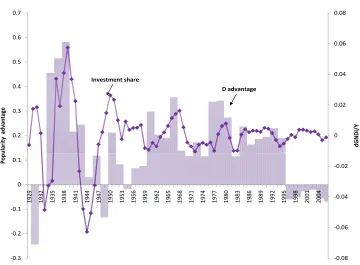
Another prediction is that as popularity advantage η goes up, the share of total expenditures
devoted to investment increases (while that of public consumption decreases). The bars in Figure
6 represent the variable Advt (described in detail in the previous section) whose changes proxy
for movements in η, the popularity advantage of the Democratic party over the Republican party
during the period 1929-2006. We can see that Democrats experienced an average advantage since the series is positive for most of the sample. Because this advantage has not been constant over time, it is possible to test our prediction by analyzing how changes in popularity affect the share of public investment.
In order to estimate the investment share as close to the model as possible, I computed it as the ratio of public investment to government spending,
Investment Share = GN DI
GN DI+GN DC,
whereGN DI stands for real non-defense public investment andGN DC for real non-defense public
consumption. Both series are obtained from the NIPA tables, and deflated by their respective deflator. Notice that I am not using government revenues or total expenditures since the model does not include debt. The investment share is HP-filtered with w=100 (due to its annual frequency), and represented by a line in Figure 6. We can see that the popularity advantage and the investment
share are positively related. A correlation coefficient of 0.25 provides support for the theory. 15
15I must note that the value ofAdv
t represents the average number of seats at theend of thetth Congress. If I
6
Concluding Remarks
I presented a model where disagreements about the composition of spending results in implementa-tion of myopic policies by the government: investment in infrastructure is too low while spending on public goods is too high. Groups with conflicting interests try to gain power in order to implement their preferred fiscal plan. Since there is a chance of being replaced by the opposition, strategic manipulation of the level of investment is optimal. In particular, the incumbent invests so as to restrict spending in the future and to maximize his group’s probability of staying in power. In contrast to previous models, the degree of ‘impatience’ of the government is endogenous here and depends on preferences and technology. The forces that drive short-sightedness are disagreement of consecutive governments, political uncertainty, and the induced lack of commitment.
I considered a case where ideological biases towards candidates from one of the groups gives them an advantage in the political arena. As a result, the voting equilibrium is asymmetric and public investment is not only inefficiently low but it also fluctuates. The group with the advantage wins elections more often becoming less impatient, so it chooses a share of investment to GDP closer to the first best. Even though both groups have symmetric preferences over the size of spending and investment, in equilibrium the group with the disadvantage tends to spend more and invest less. The political cycle is propagated into the real economy, so as parties alternate in power, different policies are implemented. In equilibrium, macroeconomic variables fluctuate even in the absence of economic shocks. Moreover, consumption, employment and output are distorted despite the fact that the government has access to lump-sum taxation.
7
Appendix
7.1 Proof of Proposition 1
The FOC with respect toK′
g is:
u1(cB(Kg), nB(Kg)) =β{pB(Kg′)VB1(Kg′) +pA(Kg′)WB1(Kg′) (16)
+pB1(Kg′)
VB(Kg′)−WB(Kg′)
+EB2(ξj′;Kg′)},
where pB1(Kg′) =
∂pB(Kg′)
∂K′
g . Denote the rule that solves this functional equation byhB(Kg)≡KB.
Define hA(Kg)≡KA analogously.
Focus on the problem of party B (and abstract from the subindexes in its value function).
ObtainV1(Kg) by differentiating equation 9 and simplifying:
V1(Kg) =u1(cB(Kg), nB(Kg))[F1(Kg, nB(Kg)) + 1−δ]. (17)
To findW1(Kg) differentiate equation (10):
W1(Kg) =u1(cA(Kg), nA(Kg))cA1(Kg) +βhA1(Kg){pB1(KA)[V(KA)−W(KA)]
+pB(KA)V1(KA) +pA(KA)W1(KA) +EA2(ξj′;KA)
, (18)
wherecA1(Kg) =F1(Kg, nA(Kg))+1−δ−xg(gA(Kg))gA1(Kg)−hA1(Kg). Notice that allocations
are evaluated given party A’s policy, because we are considering the value function of a type B
agent when his group is out of power.
Use eq. (16) to solve for W1(hB(Kg)):
W1(KB) =
1 pA(KB)
1
βu1(cB(Kg), nB(Kg))−pB(KB)V1(KB) (19)
−pB1(KB) [V(KB)−W(KB)]−EB2(ξj′;KB).
In order to replace the equation above in eq. (18) we need the value function to be evaluated in
the investment choice of government A, W1(KA). Assuming that the functions hi are invertible,
we can achieve this by evaluating eq. (19) at ˜Kg =h−B1(hA(Kg)),
W1(KA) =
1 pA(KA)
1
βuc(cB( ˜Kg), nB( ˜Kg))−pB(KA)V1(KA) (20)
−pB1(KA) [V(KA)−W(KA)]−EB2(ξj′;KA)
Replace eq. (20) into eq. (18) and simplify:
W1(Kg) =u1(cA(Kg), nA(Kg))[F1(Kg, nA(Kg)) + 1−δ−xg(gA(Kg))gA1(Kg)] (21)
−hA1(Kg)[u1(cA(Kg), nA(Kg))−uc(cB( ˜Kg)), nB( ˜Kg))].
Update eq.(21) by substituting Kg with Kg′ = hB(Kg) and replace in eq.(16). After some
manipulations obtain
u1(cB(Kg), nB(Kg)) =β
⎧ ⎨
⎩
i=A,B