DYNAMIC STRUCTURAL EQUATION
MODELS: ESTIMATION AND
INFERENCE
Dario Ciraki
London School of Economics and Political Science
University of London
UMI Number: U615888
All rights reserved
INFORMATION TO ALL USERS
The quality of this reproduction is dependent upon the quality of the copy submitted. In the unlikely event that the author did not send a complete manuscript and there are missing pages, these will be noted. Also, if material had to be removed,
a note will indicate the deletion.
Dissertation Publishing
UMI U615888
Published by ProQuest LLC 2014. Copyright in the Dissertation held by the Author. Microform Edition © ProQuest LLC.
All rights reserved. This work is protected against unauthorized copying under Title 17, United States Code.
ProQuest LLC
789 East Eisenhower Parkway P.O. Box 1346
? * * * *
S i i
-£ 5
O
Bntj©h Litr-'
-A b s tra c t
List o f Tables
2.1 Special cases of the DSEM m o d e l ... 30
2.2 T - n o ta tio n ... 32
2.3 Matrices of param eters in different model f o r m s ...64
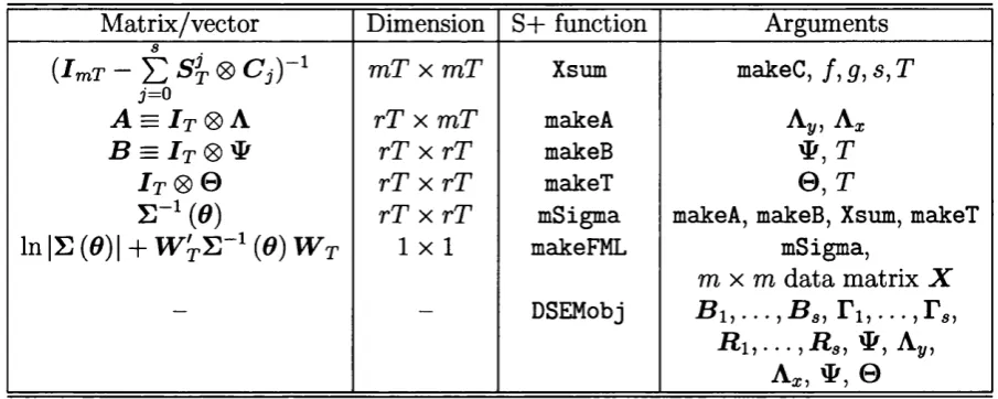
4.1 S+ functions for likelihood e v a lu a tio n ... 91
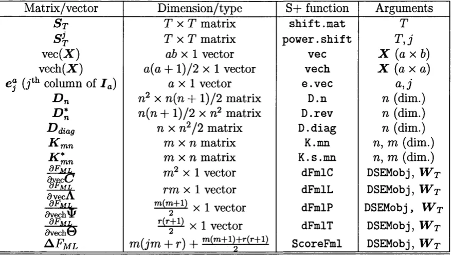
4.2 S+ functions for score e v a l u a t i o n ...103
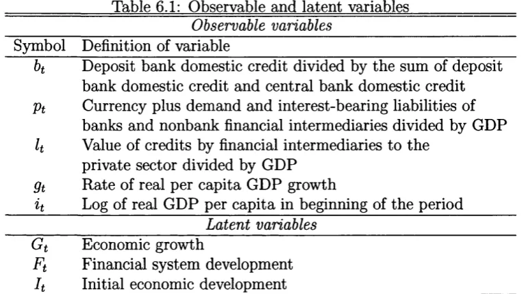
6.1 Observable and latent v a r i a b l e s ... 135
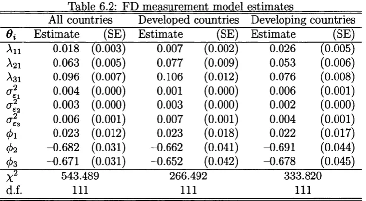
6.2 FD measurement model e s tim a te s ... 147
6.3 Country g r o u p s ...148
6.4 IV validity tests: Structural eq u atio n s... 152
6.5 IV validity tests: Measurement e q u a tio n s ... 153
6.6 FD model e stim a te s... 154
6.7 Sub-sample e s tim a te s ...155
6.8 BHPS variables used in the m o d e l... 159
6.9 D ata transform ation and variable n a m e s ... 159
6.10 Latent and observable v a r ia b le s ... 160
6.11 IV tests: BHPS m o d e l ...166
6.12 Coefficient e s t i m a t e s ...167
6.13 Variance e s t i m a t e s ... 168
List o f Figures
6.1 Empirical density of the observable v a ria b le s ... 136
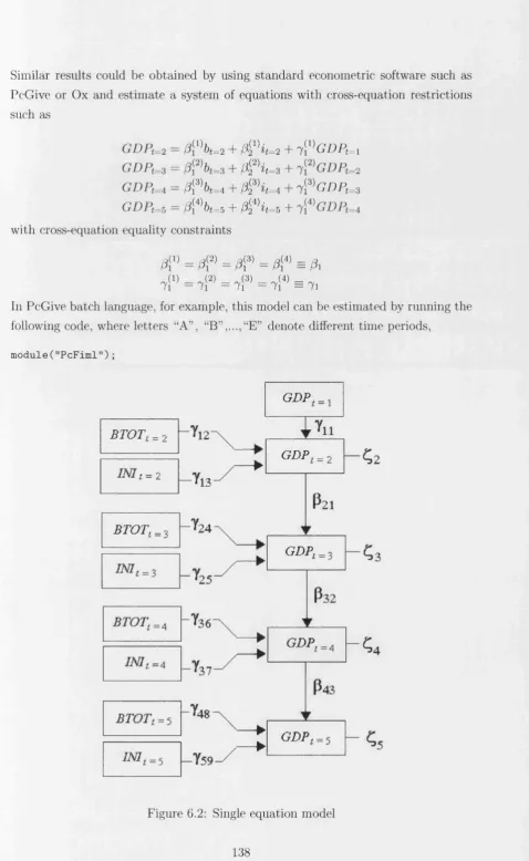
6.2 Single equation model ... 138
6.3 FD path d i a g r a m ...150
6.4 Density plot of the standardised residuals: Overall sample ...154
6.5 Density plot of the standardised residuals: S u b -sam p les... 155
C on ten ts
1 B ackground 6
1.1 In tro d u c tio n ... 6
1.2 Literature r e v i e w ... 9
1.2.1 Structural equation model ( S E M ) ... 9
1.2.2 Dynamic latent variable m o d e l s ... 11
1.3 Conclusion and aims for further r e s e a r c h ... 21
1.4 Outline of the t h e s i s ... 24
2 S ta tistica l fram ew ork 28 2.1 In tro d u c tio n ... 28
2.2 General dynamic structural equation model (DSEM) ...29
2.3 Statistical fra m e w o rk ... 36
2.3.1 Structural latent form (S L F ) ... 40
2.3.2 Reduced structural latent form ( R S L F )...41
2.3.3 A restricted RSLF ... 44
2.3.4 Observed form ( O F ) ... 47
2.3.5 State-space form ( S S F ) ... 57
2.4 Comparison of different f o r m s ...62
3 M axim um lik elih ood e stim a tio n w ith panel d ata 66 3.1 In tro d u c tio n ...66
3.2 Dynamic panel structural equation m o d e l...67
3.2.1 Maximum likelihood estim ation of the p a ra m e te rs ...68
3.2.2 Analytical derivatives and the score v e c t o r ... 74
3.2.3 Asymptotic in fe re n c e ... 81
3.3 C onclusion... 83
4 M axim um likelihood e stim a tio n w ith pure tim e series d a ta 84 4.1 In tro d u c tio n ... 84
4.2 The likelihood f u n c tio n ...87
4.3 The s c o r e ... 91
4.3.2 A numerical e x a m p le ...106
4.3.3 Conclusion... 108
5 In stru m en tal variables e stim a tio n 109 5.1 In tro d u c tio n ... 109
5.2 Generalised instrum ental variables ( G I V E ) ... 110
5.2.1 Full-sample sp e c ific a tio n ... I l l 5.2.2 Consistency conditions and instrum ental v a ria b le s...114
5.2.3 Consistent generalised instrum ental variable estim ation of the OF e q u a tio n s ...117
5.3 Full information estimation ( F I V E ) ... 120
5.4 I d e n tif ic a tio n ... 125
6 E m pirical ap p lication s 127 6.1 In tro d u c tio n ... 127
6.2 Application I: Modelling finance and g r o w t h ... 130
6.3 Application II: UK micro consumption m o d e l ...157
7 C on clusion 170 8 T echnical A p p en d ices 171 8.1 Chapter §2 a p p e n d ic e s ... 171
8.2 Chapter §3 a p p e n d ic e s ... 182
8.3 Chapter §5 a p p e n d ic e s ... 193
A cknow ledgem ents
I would like to express my gratitude to my supervisors, Dr M artin K nott for his support and guidance at all stages of this work and Professor Anders Skrondal for valuable advice and suggestions.
Further acknowledgements go to the participants of the LSE Research Seminars and colleagues from the LSE Statistics Departm ent.
Financial support and contribution from the LSE Teaching Assistantships in 2004-2006 and Departm ent of Statistics Scholarship in 2005 is also acknowledged.
C hapter 1
B ackground
1.1
Introduction
There is nothing like a latent variable to stimulate the imagination.1
A rthur S. Goldberger Latent or unobserved variables have the role of reducing dimensionality in multi variate analysis or representing quantities of substantive interest th a t are themselves not directly measurable.2 Our focus here is on structural models with latent variables where term “structural” implies specific, theoretically implied relationships among observable (manifest) and latent variables. A similar definition of structural equation models, due to A.S. Goldberger, refers to “stochastic models in which each equation represents a causal link, rather then mere empirical association” (Goldberger 1972a, p. 979).
Structural equation latent variable models (SEM) emerged from an increasingly popular but never entirely completed merger of econometric and psychometric m eth ods, namely structural or simultaneous equation models and factor analysis. The specifics and common aspects of these two traditions are reviewed in historical context by Goldberger (1972a). Psychometrics contributed factor-analytic mea surement models hence enabling empirical measurement of latent variables, while econometrics developed structural equation models th a t incorporate causal, possi bly simultaneous relationships among the modelled variables. Combined, these two approaches yield methods for modelling causal relationships among latent variables.
Joint estim ation of a classical simultaneous equations system where all mod elled variables are latent (unobserved), but measured by factor-analytic measure
1 Cited from Chamberlain (1990), p. 126.
ment models, was proposed by Keesling (1972), Wiley (1973), and Joreskog (1973). Joreskog (1973) furthermore gave a full theoretical analysis of this (general) model and pioneered its computer implementation in the still leading structural equation programme “LISREL” .
The “Joreskog-Keesling-Wiley model” (commonly known as S E M or LISREL)
can be feasibly estim ated in the full-information Gaussian maximum likelihood framework by minimising the distance between the model-implied (theoretical) and the empirical covariance matrices. Joreskog has shown th a t w ith independent, iden tically distributed (i.i.d.) Gaussian d ata the covariance m atrix has W ishart distribu tion with the known theoretical covariance structure. Hence, given the param eters of interests are identified, their maximum likelihood estimates can be obtained using iterative optimisation techniques such as quasi Newton or scoring algorithms. This does not necessarily holds for dynamic models and time series or panel data, which is likely the main reason why SEM models found considerably more applications in the psychometric and social science literature then in econometrics where dynamic models and time series d ata are standard.
Latent variables in econometrics first appeared in the “errors-in-variable” models and were broadly divided into models w ith truly latent variables and those with observable variables th a t are measured w ith error (Ainger et al. 1984, Wansbeek and Meijer 2000).
The gap between econometrics and psychometrics was partially bridged by the development of the general structural equation model w ith latent variables due to Joreskog (1973). However, dynamic structural equation models with latent variables are rarely used in the empirical literature, in contrast to the static models. This is largely due to estimation problems and lack of appropriate statistical software.
The existing methods for estimation of dynamic models in econometrics mainly focus on errors-in-variable models (Ghosh 1989, Tercerio Lomba 1990). These mod els are characterized by the assumption of unobservability due to errors in measure ment, hence the observable variables are considered as proxies containing measure ment error. This is a different and less general assumption from the one in the factor analytic tradition where the observable variables are assumed to be generated by the latent variables and thus multiple observable indicators are considered.
More complex dynamic SEM models (DSEM) using time series and panel d ata3
were not extensively researched or applied in the literature despite their considerable applicability.
In the most general framework, DSEM model encompass most dynamic linear models including dynamic simultaneous equations models, where all variables might be unobservable but measured by multiple observable indicators. Such general set ting turns out to be tedious from both theoretical and empirical side. Consequently, the literature on dynamic models with latent variables focuses on various special cases of the most general model. However, numerous substantive applications call for more general framework. The most common case th a t motivates a general DSEM model is when the relationship among the modelled variables is dynamic and simul taneous while at the same time the error of measurement (or unobservability) is present in all variables. If multiple observable indicators axe available for each un observable variable, this situation naturally leads to a dynamic SEM specification we consider here.
DSEM modelling can be used to address the problems caused by simultaneity and measurement errors in multivariate models by making use of the information contained in the observable indicators of latent, or erroneously measured variables.
In particular, we are concerned with time series and panel models th a t are char acterised by the following three points.
(i) All variables in the structural (simultaneous) model may be unobservable (la tent);
(ii) Each latent variable is measured by one or more observable indicators;
(ii) Structural relationship can be simultaneous and dynamic, thus lags of both endogenous and exogenous latent variables are possible.
In the next section (§1.2) we review the contemporary literature on structural and dynamic latent variable models and suggest th a t general DSEM models satisfying the criteria (i)—(iii) above have not been fully treated.
3We distinguish “panel” from “longitudinal” data insofar the former comprises multiple obser vations on a time series process of length T that is observed N times, while the later is made of T
1.2
Literature review
1.2.1 S tructural equation m od el (SEM )
The general structural equation model w ith latent variables (SEM) has its roots in the regression models with unobservable independent variables considered by Zellner (1970) and models discussed in Goldberger (1972b). Pagan (1973) proposed a estim ation procedure for the models with composite disturbance term s while the general structural equation model w ith latent variables, though still without multiple indicators of the latent variables was introduced by Joreskog (1973). Joreskog and Goldberger (1975) analysed a special case of the SEM model known as MIMIC (multiple-indicators-multiple-causes) which is a latent variable model with perfectly observed exogenous variables ( “causes”). Wansbeek and Meijer (2000) currently gives the most comprehensive review of the static structural equation models with the focus on the models for independent data.
The SEM model was introduced in the literature by Keesling (1972), Wiley (1973), and Joreskog (1973) and is thus also known as the Joreskog-Keesling- Wiley model The first computer implementation is due to Joreskog and Sorbom (1996b) who developed the LISREL4 computer programme (see Cziraky (2004) for a review). The basic SEM model is specified by three m atrix equations as
where 77 = (771,772, • • • ,77m) and £ = (£1,62, • • • ,£g) are vectors of latent variables,
y — (3/1»2/2, • • •, Vi) and x = (a?i, a?2, • • ■, £fc) are vectors of observable variables, and B (m x m), r (m x g), A x (k x g), and A y (I x m) axe coefficient matrices. The vectors of errors in measurement in y and x are denoted by e and 5 and assumed to be uncorrelated with 77, £, and £.
W ithout loss of generality we assume th a t variables axe measured in deviation from their mean. Note th a t (1.1) is a structural equation with latent variables and (1.2) and (1.3) are measurement models for the endogenous (77) and exogenous latent variables (£), respectively.
The specification (1.1)—(1.3), however, is not the only one and several alternatives have been suggested in the literature. The “Bentler-Weeks” and “reticular action model” specifications are the best known equivalent alternatives and both have covariance structure identical to th a t of the specification (1.1)—(1.3). Wansbeek and
4The abbreviation stands for Linear STructural RELations. 77 = B77 + T£ + C
y = Ay77 + e x = A x( + 6
( 1. 1)
(1.2)
Meijer (2000) give a more detail discussion on these alternative specifications from a comparative angle. We will use the specification (1.1)—(1.3).
Historically, the SEM model (1.1)—(1.3) emerged partly from the econometrics tradition and it is easy to see the resemblance between (1.1) and the classical econo metric simultaneous equation models. The other part came from psychometrics (factor analysis) tradition thus the measurement models (1.2) and (1.3) have a clas sical factor analytic form.
The key characteristic of the SEM model is the joint estim ation of both the struc tural and the measurement models, which is most commonly done in the covariance structure analysis (CSA) framework. There is some discussion in the literature of whether CSA should be considered as the umbrella family of methods th a t include SEM as a special case or vice versa. Originally, the method for the analysis of co- variance structures based on maximum likelihood was suggested as a fairly general approach encompassing factor analytic and related models by Joreskog (1970).
The CSA approach is based on fitting a discrepancy function th a t minimises the difference between the model-implied (theoretical) and data-implied (empirical) co- variance matrices. The SEM model (1.1)—(1.3) has a theoretical covariance structure £ (0), expressed in term s of the model parameters, of the form
=
(Ayii ( r $ r + * ) n'A', + 0 e
A yn r * A fx+ ©e5
V
A ^ r n 'A 'y +
0 £S
A s ia 's +
e s
1 ’
where I I = ( I - B ) " 1, £[££'] = $ , F[C<'] = E[eef] = © e, F[<5<5'] = 0<j, and
E[ed'] = 0 £<j. Letting z = (y' : x')' where Z = ( z i,z 2, . . . , z^r) is a sample with
N observations on z, and z = A. Zi is the sample mean vector, we can further define the sample covariance m atrix as
N
S = j - ^ ( z i - z ) ( z i - z ) ' (t 5 )
i—1
Let F ( £ (0 ) , S) be a fitting function. While the ACS method is generally appli cable to any form of £ ( 0 ), the SEM covariance structure (1.4) encompasses many common static linear models as special cases.
Most commonly used CSA fitting function used to obtain coefficient estimates th at minimise the discrepancy between (1.4) and (1.5) is the W ishart maximum likelihood function Joreskog (1981). It is given by
(GLS) and unweighted least squares (ULS) criterion (Joreskog and Goldberger 1972, Anderson 1973). The GLS discrepancy function is given by
F W P ) )o l s = (S - S ( 0 ) ) 'W - 1(S - E (0)), (1.7)
where W-1 is a general m atrix of weights. It is commonly taken th a t W -1 = S-1
in which case (1.7) simplifies to
F (E (e ))OM = l t r ( I - S - 1E (e ))2,
or if no weights are used, i.e., W -1 = I, we obtain unweighted least squares (ULS) criterion
F (E (0 ))c i s = i t r ( S - £ ( 0 ) ) 2. (1.8)
However, unlike ML and GLS the ULS criterion does not posses scale-invariance property.5 On the other hand while ML and GLS methods require positive definite covariance m atrix the ULS has no such requirement (Joreskog 1981). Note th at under some simple assumptions when plim S = £ (0o) then plim # = Oq where 0 =
a r g m in F ( £ (0), S) (Anderson 1989). The same results holds for 0 th a t minimises
F ( ' E ( 0 ) )g l s or F ( ' E ( 0 ) )u l s• In general, 0 = a r g m in F ( £ (0)) will be a consistent
estimator of Oq if F ( £ , S) —► 0 =>£ * £ -1 —►I (Shapiro 1983, Shapiro 1984, Kano 1986, Anderson 1989).
1.2.2
D yn am ic laten t variable m odels
Latent variable models specifically designed for dependent d ata (i.e. time series) were introduced in the econometric literature in the eighties and could be divided into various extensions of the classical factor analysis model and dynamic extensions of certain special cases of the static SEM model. Unlike in psychometrics, where the development of the SEM model followed an elegant path of merging the already existing simultaneous equation models w ith the factor analysis, the development of dynamic latent variable models did not follow such path. The SEM model has not been directly generalised to dynamic cases in its full generality and the factor analytic model was reoccurring in the literature often in less general settings then previously considered. In this section we give a brief overview of the main develop ments in the literature on dynamic latent variable models and show th a t most of these approaches stream from different traditions and thus fail to provide a unified treatm ent of the topic.
D y n a m ic fa c to r a n a ly s is m o d e ls
Geweke (1977), Geweke and Singleton (1981) and Singleton (1980) proposed frequency- domain methods for estim ation of a dynamic confirmatory factor model (DCFM). The DCFM model relates an observed vector x t = (xti , x t2, .. • , x tn)' to a linear
distributed lag function of a latent vector of common factors = (fti, . . . , £tk)',
and a vector of specific factors 8t = (8ti, St2, •• •, 8tn), where n > k. The model is specified as
00
* t = Y A * £ t - k + s t , ( 1 - 9 )
k=—oo
and it is assumed th a t E[x\ = 0, = 0, Cov (8it, 5jt) = 0 for i / y, Cov (<5t, £*_.,■) = 0 Vj, Cov (8t~i, 8t- j) is diagonal for i = j, and Cov(£u,€jt) = 0 Vz ^ j . Both and St are allowed to be serially correlated, and in addition can be mutually correlated.
Denoting the autocovariance function of x t by R x M = F'(xtxJ+r), for t = . . . , — 1 , 0 , 1, . . . , the autocovariance function of the DCFM model (1.9) is given by
00 00
R*(r) = Y A* Y , R «(r + k ~ 0 A 'i + «*(»•). k=—oo l= —0 0
and thus the spectral density function S x(u) can be obtained by taking the Fourier transform of H x(r), be., Sx(u;) = J2^=-oo R i W e _ M ) f°r M ^ 7r- This gives
00 00
S*(w) =
Y Y A^Y
R?(r + fc-/)A 'Ie-i^ +
Y
r= —00k= —00 l= —00 r= —00
00 00 00
=
Y
A*e~“
Y
**.(«)«>“*“
Y A'*e~"z
+
k= —00The DCFM model can be estim ated in frequency domain by firstly computing the finite Fourier transform of the vector x
x ( ^ ( T ) ) = (2irT)-1' 2 Y x teitUiiT), t=1
for j —1,2, . . . , T and ujj(T) = 2irj/T. The likelihood is given by
L ( Z ( u * ) ,S x(w'lj) = (2n) ni«|Sx(w, )| '«exp
(
- ^ x ( a ; £ ) ' S x(u>5)j ,
where uqh, h = 1, . . . , lq is the q-th band w ith lq adjacent harmonic frequencies th at splits the interval [0, ir\ into Q disjoint intervals. An unconstrained quasi-maximum likelihood estim ator of the spectral density m atrix is given by
lq
s x( u q) =
h =1
Geweke and Singleton (1981) suggest a goodness-of-fit statistic based on the likelihood ratio principle as
Sx(^ )a
S x (o;) g— X)i=l X^C-1Xi
where Sx(uj)a and Sx(a;) are unconstrained and constrained ML estim ators of Sx(<u), respectively. Asymptotically, 2 In A ~ Xd f°r d the number of distinct elements in Sx(<j) less the number of free parameters.
Note th a t Geweke and Singleton (1981) methods for estimating DCFM models are in fact based on classical Wishart-likelihood CSA approach where tim e series data is initially spectrally decomposed and “prewhitened” to eliminate seasonality and serial autocorrelation. To see the similarity with the CSA approach described in section §1.2, note th at for a finite Fourier transform of x at the m harmonic frequencies (xi, X2, . . . % ) the (complex) likelihood is of the form
x 'S x(cj)_1x ^ , thus the log of the likelihood is
InL i (Sx( o; ), xi , . . . ,5 ^ ) = —n mln(27r) — ra in |Sx(o;)| — tr C S x(o;)_1, (1-11) where C = ^ XI™ i Geweke and Singleton (1981) re-scale (1.11) by multiplying it by — m ~ l and add terms th a t do not include any unknown param eters to obtain
ln L2 (Sx(o;), xi, . . . , x m) = In |Sx(o;)| + t r C S x(o; ) _1 — In |C | - n . (1.12) Hence (1.12) is of the same form as the W ishart maximum likelihood fitting func tion (1.6). The main difference between the procedure for estim ation of DCFM models (Geweke 1977, Singleton 1980, Geweke and Singleton 1981) and the W ishart- likelihood approach (Joreskog 1970, Joreskog 1981, Anderson 1989) is in initial trans formation of the d a ta with spectral methods th a t aims at rendering d ata serially
/ m
uncorrelated and seasonality-free, thus satisfying the i.i.d. assumptions required for the CSA method. Similarly, the likelihood-ratio goodness-of-fit statistic (1.10) resembles the usual x 2 test used in the CSA framework with a transformed d ata m atrix.
An additional complication due to the use of spectral methods is th a t the Fourier transform x* generally includes complex values, hence Geweke and Singleton (1981) additionally transform the d ata vector to make it real, and similarly define real- transform of the param eter vector.
D y n a m ic m u ltip le in d ic a to r m u ltip le ca u se s m o d e l
Engle and W atson (1981) proposed a dynamic version of the MIMIC model (Zellner 1970, Goldberger 1972a, Goldberger 1972b, Joreskog and Goldberger 1975) and suggested a maximum-likelihood procedure for estim ation of a dynamic MIMIC model (DYMIMIC) .6 The model they consider is w ritten in the state-space form to facilitate application of the Kalman filer algorithm and is specified by a state and a measurement equation, respectively as
x t = (j>xt-1 + 7 zt + v t
y t = a x f + (3zt + et (1.13)
where x t (J x 1) is unobservable and y t (P x 1), and z t (K x 1) are observable vectors. The error vectors wt and e t are assumed to be normally distributed and mutually independent, i.e.,
N 0 (1.14)
R t
The DYMIMIC model (1.13) is more general then the Geweke and Singleton (1981)’s dynamic factor analysis model insofar it allows for the effects of the exoge nous variables measured without error (zt). However, (1.13) does not allow for simul taneous relationships among latent variables (xt) and also assumes th a t exogenous variables (zt) are perfectly observed. Nevertheless, the DYMIMIC model includes as special cases several im portant time series models and it can be easily shown th a t models such as ARIMA, time-varying regression models, m ultivariate ARIMA, and dynamic factor analysis are all special cases of DYMIMIC model (Watson and Engle 1983).
Engle and Watson (1981) and Watson and Engle (1983) propose an estimation approach based on the scoring algorithm and the Kalman filter. The key
cal assum ption required is m ultivariate normality and m utual independence of the measurement and state error vectors (1.14). Note th a t (1.13) can be re-written as
Yt = ol (</>xt_i + 7zt + v t) + f3zt + et
= a 0 x t_i + (c* 7 + (3) z t + ( a v t + et) ,
which now has composite error structure. If we furthermore let a v t + et = u t the model can be w ritten in term s of innovations as
u* = —a</>xt_! - (cry + (3) z t (1.15) Denoting the contemporaneous covariance m atrix of the innovations E[utu't] = Ht , it follows th a t the log-likelihood function of the DYMIMIC model is of the form
InL t {0) = - | l n | H t | - i ^ u ' f H r V (1.16) t= 1
The model param eters (0) can be estim ated recursively, using the Kalman filter, where the recursion is given by
0k+1 = 0 k + 0 k (1.17)
otf
Engle and W atson (1981) show th a t K ahnannilerjalgorithm can be applied to the DYMIMIC model when the initial state xo ls^ re a ted as either an unknown constant (fixed) or a random variable. The former assumption allows estim ation of the models containing non-stationary variables.
While relatively simple to implement, the scoring algorithm might be slow to converge thus W atson and Engle (1983) propose an additional estimation proce dure based on the expectation maximisation (EM) algorithm. The EM algorithm is particularly convenient for estimation of latent variable models because th e un known values of the latent variables can be treated as missing observations. In the DYMIMIC context, W atson and Engle (1983) implement the two steps of the EM algorithm through a m ultivariate regression (maximisation step) and by calculation of sample moments of the smoothed values of x t (estimation step). However, un like the scoring algorithm, the EM algorithm does not produce an estim ate of the information m atrix. Another problem with the EM algorithm is in its insensitivity to underidentification, thus Watson and Engle (1983) suggest th a t EM and scoring algorithms should be combined.
D y n a m ic shock-error m od el
Dynamic shock-error (DSE) model is a single equation version of an autoregressive distributed lag model w ith latent variables (Aigner et al. 1984, Ghosh 1989, Ter- ceiro Lomba 1990). In the DSE model both endogenous and exogenous variables are measured w ith error thus a static version of the DSE model is a special case of the SEM model with only one structural equation. Furthermore, the DSE’s mea surement model for the latent variables allows one observable indicator per latent variable with unit loadings. The DSE model is specified w ith a single structural equation and two measurement equations as
Vt — ^
i=1 i=l
yt = Vt + et %t — + St
(1.18) (1.19)
(1.20)
where r)t and are scalars. Therefore, (1.18) is a single equation autoregressive distributed lag model in latent variables. The variables rjt and are not observed, instead yt and x t are observed with error in the form of (1.19) and (1.2 0).
Ghosh (1989) proposed an estimation procedure for the DSE model (1.18) based on the state-space approach of Engle and W atson (1981) and Watson and Engle (1983). Ghosh (1989) and Terceiro Lomba (1990) suggest a maximum likelihood approach to estim ation of the DSE model, which would be possible if the the model could be w ritten in the state-space form (SSF).
Similarly to th e assumptions required for estimation of the DYMIMIC models, Ghosh (1989) assumes normal and m utually independent errors in the DSE model, i.e.,
i
^
to
C
t£t
i
/
0 0
\
E
£tCt
£2 £tSt
=
0
0
SfEt
.V 0 0
°8 J
The DSE model thus allows for th e measurement error in the exogenous variables, hence latent exogenous variables are perm itted in the model unlike in the DYMIMIC model of Engle and Watson (1981). However, the Ghosh (1989) model is univariate and each latent variable is measured by a single observable indicator.
N onparam etric principal com p on en ts
simple linear factor model using principal components estim ator in a “ panel” with
% = 1 , 2 , . . . , N cross-section units (or variables) observed over t = 1 , 2 , . . . , T time periods. The model is given as
( X i t ^ ( A n A12 • A ir ^ ( i u \
( 6U
\
X2t— A21 A22 • A2r & t + t
\ X N t \ A jvi AjV2 • ' A N r / \ € r t ) ^ $ N t )
where x ^ s are observed while Aij, £it and 5it are unobserved. In full-sample notation (1.2 1) can be w ritten as
X = S A + E, (1.22) where X and E are T x TV, E is T x r , and A is r x TV. This notation and terminology is somewhat unorthodox since TV denotes either the number of variables or the number of cross-section units. However, the confusion between cross-sections and variables lessens in the typical finance applications where e.g. asset returns of individual firms might be considered either as observations on individuals (e.g. different firms each with specific asset return) or as variables (e.g. different asset returns coming from specific firms), and the stock market as a whole can be seen as driven by a smaller number of unobserved factors th a t account for much of the variability in numerous observed asset returns. This nevertheless does not cover the classical panel case with both multiple individuals and multiple variables observed over a given time period.
The methods proposed by Bai and Ng (2002) typically cover m ultivariate time series models where TV denotes the number of variables, while both multiple indi viduals and multiple variables across time are not allowed, thus the model (1.21) cannot be considered a classical panel model. Note, however th a t multiple variables and multiple individuals can considered if the time dimension is absent in which case TV would denote the number of variables (e.g. types of goods) and T would denote the number of individuals (e.g. households).
Nevertheless, an im portant distinction can be drawn between classical factor analysis where either TV or T must be fixed and the model (1.21) which allows both TV and T —► oo.
The assumption in (1.21) is th a t the dimension r of the latent vector £ = (£it, £21> • • • > fri) does not depend on TV or T. There is no restriction regarding serial and cross-sectional dependence and homoscedasticity of the errors is not assumed. The degree dependence in the errors (idiosyncratic component) is however limited and in its presence the model will have an ‘ approximate factor structure’.
The key contribution of these methods relates to the situation when both TV and
likelihood estim ation methods tend to produce an estim ate of r th a t increases with
N j while the true r might be fixed in the population.
Bai and Ng (2002) estim ate the model (1.21) using the asymptotic principal component method, which minimises the criterion function
V (k, A, F*) = £ £ ( X « - A? ' ^ ) 2 . (L23)
i—1 t= 1
subject to the constraint l / N A k'Ak =
Ik
or the constraint l/T E ^ E ^ T =Ik,
wherek < m in{N , T } is an arbitrary integer. Bai and Ng (2002) proposed several non- param etric information criteria for estimating k on the basis of the principal com ponents solution.
Bai (2003) developed an inferential framework for the asymptotic analysis of the factor model (1.21) suitable for the cases when both N and T are large and when nether N nor T are fixed. In addition, Bai (2003) allows non-diagonal error covariance m atrix and serial dependence in the latent variables, which can be treated as either fixed or random, thus extending the work of Chamberlain and Rothschild (1983), Connor and Korajzcyk (1993), and Forni et al. (2000).
The contribution of the Bai (2003) is the asymptotic distribution of both the fac tors and the factor loadings. In both cases it turns out th a t the asymptotic distribu tion is normal, and to obtain this result a specific linear transform ation of factors and factor loadings was applied. In particular if we let H =
(
A ' A / N)
^ E 'S j T^j Vn t,
where E denotes an estim ate of the factor m atrix given by the y /T times the eigen vectors corresponding to the r largest eigenvalues of the m atrix X X 7, it follows th a t
plim ( S ' E / T ) = Q for an invertible m atrix Q. Subsequently, the asymptotic
T , N —yoo V / /
distribution of the linear functions y /T ( s t — H7E ^ and y /T ^A t — H7A t^ will be m ultivariate normal.
The methods suggested by Bai and Ng (2002) and Bai (2003) follow a recent tend in the financial econometrics literature on latent variable models for dependent data, however they are limited to static factor analytic models and non-param etric principal components estimation methods. Thus, the applicability of these methods to more complex dynamic models is only possibly by using the estim ated factor scores. This approach can extended to models for the non-stationary d a ta (Bai 2004), though the same limitations regarding more complex dynamic models still apply.
SE M m o d els for tim e series
ware for covariance structure analysis can be used to fit such models (Joreskog and Sorbom 1977, Jansen and Oud 1995). Longitudinal studies usually do not treat repeated measurement as stochastic processes (i.e. time series) and commonly focus on static models thereby avoiding statistical complications arising from modelling dynamic structure of the data. A as an example of a typical longitudinal model consider a sample of i = 1 , . . . , N individuals observed at two time points. Suppose
yit is brand preference and x it is personal income where we wish to estim ate a simple model of product-brand loyalty of the form
Vi2 = Oi + (3yn + 72*2, (1.24) where current brand preference {yi2) is affected by personal income and previous brand preference. This model does not treat brand preference as a stochastic process having specific statistical properties, rather it hypothesises th a t current preference toward a particular product brand might depend on the personal income but also it can be affected by person’s past brand preference.
In the simplest case with no measurement error and y and x being metrical variables we would typically estim ate the coefficient vector 0 — (a, /?,7) by ordinary least squares as 0 = (X ' X ) ~ 1X ' y2, where X = ( y 1 : ®2), Vi = (Vn, • •. ,VniY, x 2 = {x\2,. . . , x n 2)', and Y 2 = {y12, • • •, yw )'- W hen T > 2 repeated measurements
are available on the same N individuals, the usual way to arrange the d ata would be into an N x T m atrix X = ( y 1 : • • • : x t), thus X ' X ~ T x T . On the other hand, in econometric literature on panel d ata analysis it is common to stack all individuals into an N x T vector Z = {yx : • • • : x t)', which gives Z ' Z ~ 1 x 1, a scalar. The usual approach in econometrics literature is to use p repeated, lagged, values of Z
arranged as
^ yn — - \
Vi2 yn —
Vis y%2 Vi1
Ui4 Vi3 Vi 2
Vji — —
Vj2 Vji —
Vj 3 Vj2 Vji
\ 2/?4 Vjs to
where i and j are two different individuals (we assume N > T individuals are in the sample, but show matrices for N = 2 to simplify the exposition). Hence, for
Vit = PiVit + PiVit-i + A 2/it-2 + sit. On the contrary, if we arranged the d ata (for individuals i and j ) as
then computing ( W ' W ) 1W 'w* will not produce OLS estimates of the
autore-W * m atrix can be termed as “un-stacked” or “wide form at” , hence W would be the m atrix w ith “stacked” or “long form at” data.
The “wide form at” is a natural way to arrange independent d ata where each column corresponds to different variable, as it would be the case with cross-section data. Once the time dimension is introduced, the “wide form at” is still a natural if tem poral dynamics are ignored and hence if the observations taken on the same variable in different points in time are treated as different (independent) variables. Structural equation models such as those considered by Joreskog and Sorbom (1977) require an empirical estim ate of the covariance m atrix such as ( N — l ) -1 ^ fW , when N > T , though the empirical literature is inconclusive regarding SEM esti m ation when N = 1. In such case we can still compute (T — 1 but as remarked above, generally this will not lead to identical estimates.
Nevertheless, a number of empirical papers attem pted to use the covariance structure analysis as implemented in standard SEM software packages such as LIS REL to model pure time series d ata (N = 1) using (T — 1 )~l W ' W in place of the empirical covariance m atrix and using a fitting function such as W ishart likelihood. MacCallum and Ashby (1986) suggested using the SEM approach to fit time series models to cross-lagged (quasi) covariance m atrix w ith d ata m atrix arranged as
W * Vil Vi2 Vi3 Vji Uj2 Vj3
gressive coefficients computed above by (W ' W ) 1W fw . The d ata structure of the
\
V2 y i
2/3 2/2 2/1 \ 2/t 2/t-i VT-2 which after deleting rows with missing values becomes
^ 2/3 2/2 2/i ^ 2/4 2/3 2/2
Y = 2/5 2/4 2/3 (1.25)
M ultiple tim e series and lags > 2 can be arranged as a straightforward extension of (1.25). Using (1.25) to compute an empirical covariance m atrix gives
/ T f E r f
t= 3
T
E y t y t - i t= 3
T
E y t V t - 2 t= 3 T
E y t y t - i t= 3
T - l
E r f
t =2
T - l
E y t y t - i t =2 T
i E y t U t -2 \ t =3
T - l
E y t y t - i t =2
T —2
E j?
t = 1
which will converge to a Toeplitz m atrix as T —► oo for stationary time series
yt , f = 1, . . . , T .
Molenaar (1985) and Molenaar et al. (1992) considered estimation of dynamic factor models using empirical matrices such as j ^ Y ' Y . Hamaker et al. (2002) and Hamaker et al. (2003) investigated this approach to fitting univariate ARMA models and reported simulation results which implies SEM estimates differs from maximum likelihood estim ates for ARMA(p,q) models w ith q > 0. These approaches are similar to the frequency-domain methods of Geweke (1977), Geweke and Singleton (1981), and Singleton (1980) and differ in term s of whether the d ata is pre-whitened using Fourier transform or not before the covariance m atrix is computed. Further review of these and similar approaches is given in Oud (2001) and Oud (2004).
1.3
C onclusion and aim s for further research
The literature on dynamic latent variable models so far considered several spe cial cases of w hat could be seen as a dynamic generalisation of the static SEM model. Simple static factor analysis models can be estim ated under certain re strictive assumptions about the errors using static SEM methods (Amemiya and Anderson 1990, Anderson and Amemiya 1988, Browne 1984, Shapiro 1983, Shapiro 1984, Shapiro and Brown 1987).
Dynamic models in the empirical literature are primarily limited to dynamic factor analysis models (Chamberlain and Rothschild 1983, Connor and Korajzcyk 1993, Dhrymes et al. 1984, Donald 1997, Forni et al. 2000, Forni and Reichlin 1998, Geweke 1977, Geweke and Singleton 1981, Singleton 1980), or simple static factor analysis models estim ated by principal components methods (Bai and Ng 2002, Bai 2003, Bai 2004).
and W atson 1989, Stock and Watson 1998, Watson and Engle 1983, W atson and K raft 1984).
Longitudinal models or models for repeated measurement were considered in the dynamic SEM context by McArdle (1988) and McArdle (2001). A similar model was proposed by Dunson (2003) for categorical variables. These models are, however, quasi-dynamic since they treat repeated measures on the same variable as distinct variables and thus formulate standard SEM models with repeatedly measured vari ables.
The extensions th a t consider lagged exogenous latent variables or exogenous vari able measured w ith errors along with the lagged endogenous latent variables were focused on “dynamic shock-error” models and dynamic errors-in-variables models, which are essentially single equation (univariate) models with univariate measure ment models, i.e. the unobserved variables are proxied by a single indicator variable (Bloch 1989, Deistler and Anderson 1989, Ghosh 1989, Terceiro Lomba 1990). The approach taken by Ghosh (1989) and Terceiro Lomba (1990) to estim ation of the dynamic shock-error models is based on their re-writing in the state-space form. However, even w ith the simplest univariate models the state-space form is difficult to obtain. Ghosh (1989) solves this problem by introducing an additional autore gressive equation for the exogenous latent variable. On the other hand, Terceiro Lomba (1990) considers models with contemporaneous exogenous latent variables hence avoiding the problem w ith lagged exogenous variables which cannot be easily w ritten in the state-space form.
The existing literature is scarce in respect to dynamic structural equation model w ith latent endogenous and latent exogenous variables, multiple simultaneous equa tions, and measurement models for the latent variables w ith multiple indicators. Such models would present a dynamic generalisation of the static multi-indicator SEM model, hence, theoretical and practical consideration of dynamic SEM models would be an im portant extension of the literature.
In summary, we can identify three main problem areas where further research is needed.
Unifying theoretical framework Different traditions in the literature deal w ith vari ous special cases of dynamic structural equation models, such as errors-in-variables, state-space, and latent variable models. There is a notable divergence in the liter ature and lack of cross-referencing. Consequently, methods th a t focus on errors-in- variables, latent variable models, or state-space models appear to be concerned with different models rather then special cases of dynamic structural equation models.
difficult or impossible to obtain for complex m ultivariate models such as DSEM using standard methods.
1.4
O utline o f th e th esis
The thesis focuses on estim ation of dynamic structural (i.e. simultaneous) equation models in which some or all variables might be unobservable (latent) or measured w ith error. Moreover, we consider the situation where latent variables can be mea sured w ith multiple observable indicators and where lagged values of latent variables might be included in the model. This situation leads to a dynamic structural equa tion model (DSEM), which can be viewed as dynamic version of the structural equation model (SEM). Our focus is on obtaining coefficient estimates using both param etric and non-parametric methods. Post-estim ation diagnostics and measures of overall fit are beyond the scope of the present work and are thus left for further research.
Taking the mismeasurement problem into account aims at reducing or elimi nating the errors-in-variables bias and hence at minimising the chance of obtaining incorrect coefficient estimates. Furthermore, such methods can be used to improve measurement of latent variables and to obtain more accurate forecasts.
The literature on dynamic latent variable models can be divided into several different traditions emerging from fields such as econometrics, psychometrics, and engineering. Certain special cases of dynamic structural equation models, such as dynamic factor model, have been extensively analysed in the time series literature. There is a close link between these methods and the unobservable states models estim ated in the state-space form. In chapter §1 we give an overview of the literature by addressing the key developments and pointing out to the areas requiring further research.
Latent variable models have been traditionally analysed as errors-in-variable models using instrum ental variables methods in the mainstream econometrics liter ature, as covariance structure models in the psychometrics literature, and as state space models in both engineering and econometrics literature. Chapter §2 addresses the a lack of a unifying theoretical framework for dynamic models w ith latent vari ables and suggests such framework based on DSEM model, which can be shown to encompass numerous specific models considered in the literature. The approach taken here uses the idea of a Gaussian vector likelihood and specifies the theoreti cal covariance structure implied by the DSEM model for a m ultivariate time series process th a t started at t = 1 and was observed till t = T. It is shown th a t differ ent approaches to errors-in-variables and latent variables can be viewed as different forms of the DSEM model, hence giving rise to specific m ultivariate likelihoods, whose param etrisations can be compared within a unifying statistical framework.
pressions for the score and the Hessian m atrix along with a closed-form (theoretical) covariance m atrix. The closed-form covariance m atrix is obtained by making cer tain assumptions about the pre-sample values, which requires large-T asymptotics. Some of the existing theoretical results for the SEM model, namely the analyti cal first derivatives, were implemented in SEM software packages such as LISREL, which can be used to estim ate certain DSEM models for panel d ata with relatively small T.
The analytical results obtained in chapter §3 differ from the existing results in two respects. Firstly, the model is formulated for the time series process, which eliminates the necessity to specify a separate SEM model for each tim e point and then impose cross-equation restrictions across all tim e points, as it is necessary in LISREL and similar SEM software packages. Secondly, the analytical results are obtained using modern m atrix calculus methods based on zero-one matrices th at enable derivation of fully vectorised expressions for the first and second derivatives. Moreover, the obtained score vectors contain derivatives for individual DSEM coef ficients thus no equality or symmetry restrictions need to be imposed on the score vector. Fully vectorised expressions make standard asymptotic analysis straightfor ward and facilitate computer implementation in modern m atrix languages such as S, R, or Ox.
Chapter §4 considers maximum likelihood estimation of DSEM models w ith pure time series d ata using a “raw d ata ” maximum likelihood (RD-ML). In this chapter we obtain the closed-form expressions for the likelihood and analytical derivatives of the pure time series DSEM model thus providing the analytical inputs for the RD-ML estimation. Moreover, we outline some S code for estimation of such models using quasi-Newton optimisers in S-Plus and R environments.
In chapter §5 we propose non-parametric methods for estim ation of DSEM mod els suitable for both pure tim e series and panel data. Generalised instrum ental variables (GIVE) and full information instrum ental variable (FIVE) methods are considered for the estim ation of DSEM models in the “observed form” , i.e., as errors- in-variable models with composite error terms.
ments. Empirical validity of such instrum ents can be tested using standard validity of instrum ents tests. Instrum ental variables methods have a well known advantage of not imposing any distributional assumptions on the data. They also provide non iterative estim ators th at are very easy to compute using standard general purpose statistical software. An additional purpose of these methods is in obtaining good starting values for maximum likelihood estim ation using standard SEM software packages such as LISREL.
In chapter §6 the above methods are applied to real-data empirical examples with two main aims. The first aim is to dem onstrate how DSEM models can be estim ated using standard econometric and SEM software packages when starting values are obtained using the methods suggested in chapter §5. Both fixed and random effects dynamic panel models are considered in the context of specific empirical applications: a model of financial development and economic growth and a micro-consumption model. The second aim is to investigate the limits of the existing SEM software on data size and model complexity in estim ation of empirical DSEM models.
DSEM models can be easily estim ated using G IV E/FIV E methods w ith stan dard econometric software packages, which holds for both pure time series and panel models and for very large d ata sets. Moreover, these methods provide estimates th a t can be used as starting values in standard SEM software packages. Using the LIS REL package, we show th a t even for relatively simple DSEM models convergence cannot be achieved without starting values th a t are very close to the maximum likelihood estimates. Nevertheless, we show th a t the starting values obtained with G IV E/FIV E methods can be successfully used as starting values in LISREL esti mation.
The ability of SEM software to handle panels w ith large T is, however, very limited. Along w ith the need to specify the model for each time point and subse quently impose equality constraints on all param eters across T tim e points, we also report computing difficulties associated even w ith relatively small T. The largest model we estim ate using LISREL in combination with G IV E/FIV E starting values uses a panel d a ta set w ith N = 5152 and T — 13. Using these data, we estim ate a DSEM model with three structural equations including dynamics of up to five lags, with 37 coefficients, estim ated as 13 x 37 coefficients with equality constraints across T = 13 time periods, which might be one of the largest models estim ated with LISREL. It seems unlikely th a t similar models could be estim ated for much larger
T using standard SEM software such as LISREL. This suggests two limitations of the currently available SEM software for estim ation of panel DSEM models. First is dependence on externally provided starting values. The second is the “small T
C hapter 2
S ta tistica l fram ework
2.1
Introduction
The literature on dynamic latent variable models can be broadly classified into three traditions. The first tradition emerged from econometrics literature on the errors-in- variable models and regression with measurement error (Cheng and Van Ness 1999, Wansbeek and Meijer 2000). The second one is closely linked to covariance structure m ethods and generalised m ethod of moments, streaming from the psychometrics and m ultivariate statistics (Joreskog 1981, Bartholomew and K nott 1999, Skrondal and Rabe-Hesketh 2004). Finally, the third tradition based on estimation of the models w ritten in “state-space form” emerged from control engineering and was adopted in econometrics owing to the suitability of the Kalman filter algorithm for estimation of various econometric models w ritten in the “ state space form” (Harvey 1989, Durbin and Koopman 2001).
This threefold and apparently diverging developments did not facilitate advance of dynamic latent variable models matching the expanding literature on static latent variable models (see e.g. Skrondal and Rabe-Hesketh (2004) for a comprehensive review). Consequently, specific empirical applications became linked with particular estim ation methods and a lack of a more general framework hindered estimation of more elaborate empirical models. For example, the DYMIMIC model of Engle et al. (1985) perm its dynamics in the endogenous latent variables but does not allow exogenous latent variables, which facilitated a number of empirical applications in which substantive problems had to be limited to static, perfectly observable exoge nous variables.
We suggest a unifying statistical framework for dynamic latent variable models based on the general dynamic structural or simultaneous equation model (DSEM). DSEM model is general in the sense it subsumes many dynamic (and static) linear models under a common param etric form.
We develop a statistical framework by making distributional assumptions about the exogenous components and the measurement errors in the general DSEM model. We then show how the general model can be formulated following the three main traditions and compare the models resulting from such formulations by referring to their stochastic properties. In particular, we show th a t different approaches do not necessarily result in identical reparam etrisation of the general model, rather some additional or different statistical assumptions need to be made to make different models equivalent. Finally, we suggest th a t some forms are suitable for particular estim ation methods and briefly discuss the implications for the development of such methods.
2.2
G eneral dynam ic structural equation m odel
(D SE M )
In this section we consider a dynamic simultaneous equation model with latent variables (DSEM). A DSEM(p, q) model at any time period t using the “ t-notation” as
r,t = ^ r £ t - j + <t (2-1)
3 = 0 j= 0
V t — A y T I t + £ t ( 2 - 2 )
Xt = A x£t + &t (2*3)
where r)t = (^(1), r ) f \ . . . , ?yt(m))' and £t = (ft(1),&(2), . . . , &(9))' are vectors of possibly unobserved (latent) variables, y t = . • •, y\n^Y and x t = (x x f \ . . . , x[k^)'
are vectors of observable variables, and B j (m x m ), r j (m x g), A x(k x g), and Ay
(n x m ) are coefficient matrices. The contemporaneous and simultaneous coefficients are in B0, and jTo, while Bx, B 2, . . . , B p, and JTi, r 2, . . . , F q contain coefficients of the lagged variables.
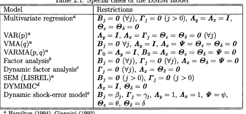
restrictions on its param eter matrices. Table 2.1 lists the most common multivariate models and shows how they can be specified as special (restricted) cases of the general DSEM model (2.1)-(2.3).
________________ Table 2.1: Special cases of the DSEM model________________
Model Restrictions
M ultivariate regression0
VAR(p)° VMA(g)° VARMA (p, q)a
Factor analysis6
Dynamic factor analysis0
SEM (LISREL)0
DYMIMICd
Dynamic shock-error model6
B j = 0 (Vj), = 0 {j > 0), A y = A x = 7,
0 £ = 0 s = 0
A y = 7, A x = 71,- = 0 £ = 0 5 = 0 (Vj)
B j = 0 Vj, A y = 7, A x = & = 0 £ = 0 5 = 0
To = A y = 7, Bo = A x = 0 £ = 0 s = & = 0 B j = 0 (Vj), T j = 0 (Vj), A x = 0 s = V = 0 r j = 0 (Vi), A x = 0 s = 0
B j = 0 ( j > 0), = 0 ( j > 0)
A x = 7, 0 s — 0
B j (3j, T'j Ay 1, A x 1, “0,
e £ = 9 , 0 8 = 5 a Hamilton (1994), Giannini (1992).
6 Bartholomew and Knott (1999), Skrondal and Rabe-Hesketh (2004). c Geweke (1977), Geweke and Singleton (1981), Engle and Watson (1981).
d Engle et al. (1985), Watson and Engle (1983). e Ghosh (1989), Terceiro Lomba (1990).
The idea behind the SEM model was to combine multiple-indicator factor-analytic measurement model for the latent variables w ith a structural equation model thus al lowing for the measurement error in all variables in the structural model (Joreskog
1970, Joreskog 1981, Bartholomew and K nott 1999, Skrondal and Rabe-Hesketh 2004). The static SEM model can be w ritten as a special case of (2.1)—(2.3), i.e.,
Vt — B 0rjt+ To£t + Ct (2-4)
Vt = AyVt + et (2.5)
x t = + (2.6)
Since both rjt and £t are unobservable some reduction or elimination of the unob servables would be necessary. An econometric interpretation would consider (2.4) a simultaneous equation model in the structural form (see e.g. Judge et al. (1988)). Here, by “ structural” we refer to the model with endogenous variables on both sides of the equation as opposite to the “ reduced” model, which has endogenous vari ables only on the left-hand side. We can easily obtain the reduced form of (2.4) as1
rjt = ( I — B0) - 1 ( r 0£t + £t), which can be further substituted into (2.5) to obtain the “ reduced ” form of the model
[image:34.595.27.446.176.370.2]Vt — Ay ( I — Bo) 1 (r o £ t + £f) + et
= A x£t + St,
(2.7)
(2.8)
with has only observable variables on the left-hand side. This enables derivation of the closed-form covariance m atrix of W{ = (y't : x [)' in terms of the model param eters. For instance, if Wi ~ N (fjt, 27), it follows th a t (T — 1)S ~ W (T — 1,17), where S = 5Z*=i w iw i *s the empirical covariance m atrix, and W denotes the W ishart distribution.2
However, the same approach cannot be straightforwardly applied to the DSEM model (2.1)-(2.3), which contains lagged latent variables. Namely, the reduction from (2.4)-(2.6) to (2.7)-(2.8) would not eliminate the lagged values of rjt .
The likelihood function for a sample of T observations generated by a dynamic model specified for a typical tim e point t (i.e. in “ ^-notation), such as (2.1)—(2.3), can be obtained recursively by sequential conditioning (Hamilton 1994, p. 118). In this approach we would write down the probability density function of the first sample observation (t = 1) conditional on the initial r = max(p,q) observations and then obtain the density for the second sample observation (t —2), conditional on the the first, etc. until the last observation (t = T ). The likelihood function would then be obtained as a product of the T sequentially derived conditional den sities, assuming conditional independence of the successive observations. However, this approach is not feasible for complex m ultivariate dynamic models with latent variables as sequential conditioning soon becomes intractable.
An alternative approach leading to an equivalent expression for the likelihood function would be to assume th a t the observed sample came from a T-variate (e.g. Gaussian) distribution, having multivariate density function, from which the sample likelihood immediately follows (Hamilton 1994, p. 119). This approach might not be easily applicable to dynamic latent variable models for which we generally wish to obtain the likelihood in separated form, i.e., w ith all unknown param eters placed in the covariance m atrix, separated from the observed d ata vectors. W ithout such
2 The Wishart distribution has the likelihood function of the form
JW ) p
7 r i r ( r- i ) 2 i ( T ( n + f e ) ) | 2 7 | i ( " + f e ) f ] p ( T + i ~ j )
j=i V 7
separation we would be left w ith T “missing” observations on the latent vectors rjt
and £t instead of only their unknown second moment matrices.
We can solve this problem by specifying a DSEM model (2.1)-(2.3) for the time series process th a t started at time t = 1 and was observed till time t = T using a “ T -notation” defined in Table 2.2. The vector {*}^ can then be taken as a single realization from a T-variate distribution.
Table 2.2: T-notation
Symbol Definition Dimension
H t v e c f a j 'f = (*?!> • • ? Vt) m T x 1 Zt vec{C t}[ = (Cl,-- ,C r)# m T x 1
/ji v e c { £ j [ = (Cl), • • g T x 1
Y t vec {ytY i —(2/1, - * , Vt) n T x 1
Et vec {et}i = fal,-- , e't) n T x 1
X t vec { x t}i = ( * ! ,.. , x'T) k T x 1 At vec {<5t}^ = ((51,.. ,#t)' k T x 1
Working w ith the model in T-notation will enable us to “ reduce” the model (2.1)-(2.3) and obtain a closed form covariance structure and hence a closed form likelihood of the general DSEM model.
We make the following simplifying assumption about the pre-sample (initial) observations.
A ssu m p tio n 2.2.0.1 (In itial ob servation s) We assume that r = max(p, q) pre sample observations are equal to their expectation, i.e., = 77j(_r+1) = ••• =
Vio 0 and 0 .
Anderson (1971) suggested th a t such treatm ent of the pre-sample (initial) values allows considerable simplification of the covariance structure and gradients of the Gaussian log-likelihood. More recently, Turkington (2002) showed th a t making such assumption allows more tractable mathem atical treatm ent of complex multivariate models by using the shifting and zero-one matrices. In addition, we require covari ance stationarity as follows.
A ssu m p tio n 2 .2 .0 .2 (C ovariance sta tio n a rity ) The observable and latent vari ables are mean (or trend) stationary and covariance stationary.
Letting s = . . . , — 1 , 0 , 1, . . . , we require the following 1. E [„ t] = E K J = 0 =► E [ y t] = E [ xt] = 0 ?
[image:36.595.103.364.223.367.2]2. The structural equation (2.1) is stable, and the roots o f the equations
I - X B r - A2B2 --- ApjBp| = 0 and \ I - A A - A2T2---\ « r q\
=
0By Assumption 2.2.0. 2 it follows th a t the observable variables generated by the latent variables are also covariance stationary, i.e., Vs, k G Z, E [yty !t_s ] = E [yty't_k] , E = E , and E [ytx't_g] = E • N ext> by Assumption
2.2.0. 1 the pre-sample (initial) observations are zero thus we can ignore them and write the DSEM model (2.1)-(2.3) for the tim e series process th a t started at time
t = 1 and was observed until t = T in the “ T-notation” as { q t }^ = (rj1, . . . ,?7T), or
and similarly, = (£1?. . . , £T) and {C t\i = (Ci> • • •»Cr)- The structural equa tion (2.1) can thus be w ritten for the time series process as
using the vec operator th a t stacks the e x / m atrix Q into a n e / x 1 vector vec Q, are greater then one in absolute value.
3. E [& £ _ ,] = $ s, so that $ - s = &s.
(2.9)
V Q
{»»«}[
= Y s B ifottf
S 't+ E
r > S 't+ {<*}
T
1 ’ (2.10)
where we made use of a T x T shifting m atrix St given by / 0 0
1 0
St = 0 1
0 o \
0 0
0 0 (2.11)
\ 0 ••• 0 1 0 /
By definition, we take = It- The structural equation (2.10) can be vectorised