APPLICATION OF FITNESS SWITCHING GENETIC ALGORITHM FOR SOLVING 0 1 KNAPSACK PROBLEM

7599

QUERYING RDF DATA

1,*_{ATTA-UR-RAHMAN,} 2_{FAHD ABDULSALAM ALHAIDARI}

1,*_{Department of Computer Science,} 2_{Department of Computer Information System} College of Computer Science and Information Technology,

Imam Abdulrahman Bin Faisal University, P.O. Box 1982, Dammam, Kingdome of Saudi Arabia.

Email: aaurrahman,faalhaidari}@iau.edu.sa

ABSTRACT

Resource Description Framework (RDF) is a data model to represent and store the web contents and their association in the form of a graph. This will enable the web (semantic web) to answer queries in a meaningful way as compared to the current web of keyword locator. Querying is required to retrieve any information from the semantic web (RDF data). In this context several algorithms have been proposed which can be classified in different categories. There are mainly two ways to query RDF data, one ‘on the fly’ and the other is ‘index query’. The indexing method requires lot of offline work on RDF data to make the query run faster over it but at the cost of increased space. On the other hand, the ‘on the fly query’ algorithms’ takes more time to execute. In this research, an algorithm with reduced time and space complexity is proposed. The data graph is being stored in an Adjacency Matrix and Adjacency List. Our algorithm tries to match the query graph with the data graph (graph pattern matching) with lesser cost. By comparing the results, it is observed that proposed technique’s results are more accurate with reduced complexity.

Keywords: RDF, Graph Data Query, Semantic Web

1. INTRODUCTION

RDF (Resource Description Framework) is a basic data model used to represent resources and to represent information of resources in the web. The RDF can be representing in graph form and has attracted the attention of many researchers. Hence, many researchers have devised different methods to store and query RDF data. Some of the techniques store RDF data in Relational Databases i.e. (Y. Yan, 2009) [1] used the triple stores to store the RDF triples and has reduced the join cost, (Akiyoshi Matono, 2005) [2] gave the idea of path queries and handled the RDF schema as well, (Shady Elbassuoni, 2011) [3] gave the idea of keyword queries. There are also RDF databases to store and query RDF, one of the RDF database that base on indexing scheme is the HPRD (High performance RDF database) (Baolin Lui, 2010) [4]. The one of other indexing scheme is use of Suffix Array (A. Matono, Sept. 2003) [5] (Kim, Sept. 2009) [6], the Suffix Array is used to index the all paths and then the query is applied. Rest of the paper is organized as follows. Section 2 contains the related work, section 3 explains the proposed work. Section 4 contains case studies to show performance of the proposed scheme and section 5 concludes the paper.

2. RELATED WORK

This section contains the review of some well-known techniques for querying the RDF data with their features.

7600 2.2 Graph Partitioning in RDF Triple Stores

Yan et al. (Y. Yan, 2008) [7][1] introduced a new method to store, index and query RDF data. In this technique the focus is on the graph form of RDF data. The mature Relational database has been used, called triple store (Anon., 2013) [8] to store the RDF. Firstly, they partition triples of RDF Graph into overlapped sub graphs and add one more column that represents Group ID in triple table. Group ID, is used to identify sub graph represented by an integer value. Then, the partitioned triples are stored in the table according to grouping, the Group ID column tell about in which group the desire triple resides. The advantage for doing this is that now the SPARQL query (Anon., 2013) (Hutt, 2005) [9] be applied group wise on the table hence decreasing the join cost much. A query is first divided into multiple simpler queries and then applied over the table to RDF groups.

2.3 Indexing Approach using Suffix Array Matono et al. (A. Matono, Sept. 2003) proposed an indexing approach to store RDF data and RDF Schema by using Suffix Array (Manber, 1993) [10] to process the path queries. Suffix Arrays, are the known data structure used for textual search. It is a one-dimensional character string that contains only indices of the textual data. In this paper, Firstly, from the RDF data four DAGs (Directed Acyclic Graphs) have been extracted and then all paths expressions have been extracted from DAGs and Suffix Array for all extracted path expressions has been created. The used an algorithm to extract path expressions. This algorithm traverses every root vertex of RDF Graph and gives all possible path expressions. The Time Complexity of this algorithm is O (|R| |E|) time.

2.4 Processing of Path Queries Using Suffix Array

In this paper (Kim, Sept. 2009) [6], Kim proposed an improved indexing and query processing approach to improve the performance of Matono’s approach (A. Matono, Sept. 2003). In this paper some of the problems in the (A. Matono, Sept. 2003) has been highlighted and fixed. The one of the major problems was, Matono et al. deleted the repeated suffixes due to which many of the backward queries missed some results. To handle this problem Kim suggests not deleting the repeated suffixes. Further Kim has proposed new indexing approach and computed the LCP (Longest Common Prefix) along each suffix to reduce the repeated pattern matching. Kim has created several Suffix Arrays instead of one by separating them according to their start value and store these start values in separate array called

‘keywords’. The keywords Array is connected to two arrays, one Suffix Array and another LCP Array. Now the path expression of the query will be searched in keywords Array with reduced cost instead of whole Suffix Array as in Matono’s approach. The LCP Array is used to search for the other suffixes that are same as path expression. As it contained the common prefix of last Suffix Array of itself, hence there is no need to perform repeated pattern matching over first matched Suffix Array. This reduced the cost of time consuming pattern matching. To process the Query an algorithm devised that can return the query result in O(log n) time.

2.5 High Performance RDF database (HPRD) Baolin Liu [4] & Bo Hu [20] has introduced a high-performance storage system for RDF data in HPRD. They have used indexing approach and worked of query evaluation. HPRD combines different techniques of other databases. Three types of indices Triple index, Path index, and Context index have been used in HPRD. In HPRD the nodes of RDF Graph are index with increasingly monotonically assigned OIDs (Object Identifiers), this makes the processing over nodes (e.g. comparison) easy and saves time (as OIDs are smaller than nodes labels itself). Triple index has been used for the efficient retrieval of the triples. The RDF Graph is divided into four subgraphs to manage the semantic information and maintain indexing for each subgraph, i.e., schema graph, class graph, property graph, general resource subgraph. For each subgraph the indexing is maintained e.g. Schema index for schema data to answer the class and property based queries, Class index for hierarchy of class, Property index for hierarchy of property etc. A heuristic based algorithm is used to select for a specific strategy, a join order selection is needed. The algorithm tries to make the interval result set against the join processing as small as possible through statistical analysis over triple patterns.

2.6 Summary

7601

3. PROPOSED WORK

A new method to store and query RDF data is proposed, depending on the nature of data (if graph is dense then the Adjacency Matrix and if graph is sparse then Adjacency Lists). To get an efficient solution to the problem of Querying RDF data, we have gone through different stages, described next.

3.1 Storing RDF data using Adjacency Matrix Firstly, the RDF data is stored in the form of Adjacency Matrix (Morin, 2012) [11]. The Adjacency Matrix is a nxn matrix (where n is number of nodes), with rows and columns labeled by graph vertices. Adjacency Matrix describes a graph by representing which vertices are adjacent to which other vertices, the cell of Adjacency Matrix is filled with the label of the edge. There are already ways to store RDF data (David C. FAYE, 2012) [12]. 3.1.1 Creating Adjacency Matrix

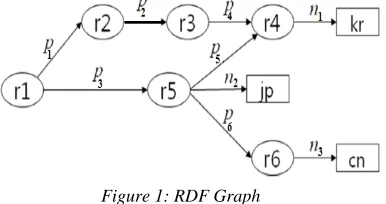
We have considered a small RDF Graph given in Figure 1, as an example to show the functioning of our technique. This RDF Graph is a representation of RDF data, where nodes represent the ‘Subjects’ & ‘Objects’ and edges’ label represent ‘Property’. The ovals in graph in Figure 1 are resources and the square are the literals. This small RDF Graph when stored in Adjacency Matrix is shown in the Figure 2. As there are 9 nodes in graph hence Adjacency Matrix create against it is a 9×9 square matrix. We put nodes on the both sides of Matrix. To fill Adjacency Matrix, the name of nodes at row and column is checked. If nodes are connected then the label of the edge is written in the corresponding matrix’s cell, else “0” is written. For our convenience 0’s is omitted for clarity.

Figure 1: RDF Graph

Consider the Query given in the Figure 3, in the RDQL format (Seaborne, 2004) [13]. This query will retrieve all those resources which are reachable from a given path pattern given in the query in the form of series of triples. The Path Pattern is the condition in the ‘where clause’ of the above query that is, 'r1.p3.r5.p5.?x'.

Figure 2: Adjacency Matrix of RDF Graph

Figure 3: Query

The path pattern can be represented with the graph and is called Query Graph. The Query Graph for the above query is given in the Figure 4. As the last node is unknown i.e. what resource is it (it will be retrieved by processing the query) so it is left blank to make prominent.

Figure 4: Query Graph

The Adjacency Matrix for the Query Graph can be created in the same way as for RDF Graph. First, the number of nodes are extracted, as there are 3 nodes and hence 33 matrix will be created and filled accordingly. The Adjacency Matrix for the Query Graph is shown in the Figure 5.

Figure 5: Query Adjacency Matrix

3.1.2 Query Processing

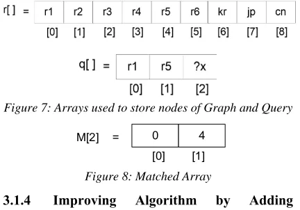
7602 not yet compared and its corresponding nodes will be searched from the Adjacency Matrix of RDF. These nodes will be the answer to the query. The Algorithm shown in the Figure 6 is used for answering the query. Two 1-D Arrays are used to store the nodes of RDF and Query Graph. As seen in Figure 7, r [9] is used to store nodes of RDF Graph (Figure 1) and q [3] is used to store the nodes of Query graph (Figure 4). The q [], stores all the nodes of query graph and r [] stores the nodes of RDF Graph. The Algorithm1 (Figure 6) has three parts. First part compares r [] & q [] and stores the index of r [] in M [], a matched Array. For example, for r [] & q [] given in Figure 7 the Matched Array is shown in Figure 8.

Figure 6: Algorithm for Query Processing

The second part of Algorithm 1 uses these indices of M[] to compare R[][] and Q[][] (2-D arrays to store RDF Graph and Query Graph respectively). The Algorithm exit when query’s triple is not found. The third part of the Algorithm is used to find out the resulting resource. This part uses a for loop and

iterate through every node of RDF Graph to find out the desired resource.

3.1.3 Time and Space Complexity

The Time Complexity of this algorithm is O(m×n) but the Space Complexity is O(n2), where m is the number of nodes of Query Graph and n is the number of nodes in RDF Graph. This Algorithm handles the path queries (Forward Path Query). Path query is such a query in which a path is given in the form series of triples and a part of it needs to be found. Considering the first part of the algorithm, there is loop run over the all nodes of the RDF Graph. If the graph is large then this will take more time to search the relevant node. To find out the index (of matched resource) in the RDF nodes, we can apply hashing which will give index of the desired node in constant time. However, an extra space will be used there but efficiency will be improved a lot. The collisions will not occur as Minimal Perfect Hash Function (Anon., 2012) [14-18] is used (each key can be retrieved from the table with a single probe). Hence, this will save the storage and decrease the Time Complexity, too.

Figure 7: Arrays used to store nodes of Graph and Query

0 4

= M[2]

[0] [1]

Figure 8: Matched Array

3.1.4 Improving Algorithm by Adding Hashing

7603

Figure 9: Algorithm using Hash Map

Figure 10: Hash Map

The time complexity of the algorithm 2 is O(m×n), where m is the number of Query Triples and n is the number of nodes in the RDF Graph. In the procedure findresource(), the Algorithm 2 iterates through all the nodes of the RDF Graph to find out the missing object of the triple (this Time Complexity is in worst case). As the RDF Graph is made up of millions of nodes and to search for a specific property against each node will have to search for the all the nodes of the Graph and will take time. Hence there is a dire need for such a solution that can reduce this search. The solution to this problem is to use another Adjacency Matrix for the property, which is further discussed in the next session.

3.1.5 Improving by using Property Adjacency Matrix

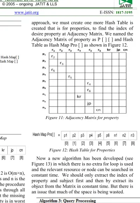
Algorithm-2 there is another extra for loop being used to search for the desired resource (line 17 to 22). This loop will run number of RDF Graph’s nodes times in worst case. To handle the issue of Time Complexity, one more Adjacency Matrix for properties will be used shown in Figure 11. At its row side the properties are placed and the subject of property will be given on the column side. The Adjacency Matrix will be filled with the object of property (that can be approached through that property). In this way the desired node can be answered in constant time. To implement this

approach, we must create one more Hash Table is created that is for properties, to find the index of desire property at Adjacency Matrix. We named the Adjacency Matrix of property as P [ ] [ ] and Hash Table as Hash Map Pro [ ] as shown in Figure 12.

Figure 11: Adjacency Matrix for property

Figure 12: Hash Table for Properties

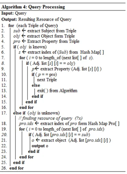
Now a new algorithm has been developed (see Figure 13) in which there is no extra for loop is used and the relevant resource or node can be searched in constant time. We should only extract the index of property and subject first and then by extract its object from the Matrix in constant time. But there is an issue that much of the space is being wasted.

Figure 13: Algorithm using Adjacency Matrix of Property

7604 notice that Time Complexity has reduced to its most extent. Now to search for the specific object connected with property it does not need to iterate through all the nodes. The Adjacency Matrix of property will provide the missing object. No doubt, this has increased the Space Complexity. Space Complexity has doubled the Space Complexity of Algorithm-2. Here it can be seen that much of the cells of the Adjacency Matrix are not used as with a specific property there can’t be very large number of nodes. Further, it can also be noticed that most of the cells are not being used and high space is used for a simple RDF Graph. Considering the real time RDF Graph then lot of space would be required. As a solution to this aspect, Adjacency Lists are used.

3.2 Storing RDF data using Adjacency List Due to Adjacency Matrix lot of space is used, hence as a solution Adjacency Lists are used. 3.2.1 Creating Adjacency List

By using the Adjacency Matrix, the Path queries in a linear time can be answered but there is lot of space used in it. To save the space Adjacency Lists [19] have been used. The example graph stored in Adjacency List shown in the Figure 14. Adjacency List of graph properties is also produced in a way that, Master List of all the properties is produced and the Subjects and Objects adjacent to those Properties are stored in next Adjacent List (in Figure 15). 3.2.2 Query Processing

It is quicker to find out if there is an edge between two vertices using an Adjacency Matrix (only should look at one item), but in an adjacency list we must look at all items in a node’s next list to see if there is an edge to another node. Hence, as we have reduced the space but the Time Complexity will be lost (but little). One more for loop to find the desired property in the node’s adjacent lists will have to be used, which will make the Time Complexity to two nested for loop, but these two for loop are not much longer. The Algorithm shown in the Figure 16 is used to answer the query. It extracts each triple and then extract subject, predicate and object of the triple and start searching the path query. For each triple, it first finds the subject in Master Adjacency List. To quickly find the subject the Hash Table will be used and the in that desired subject it will find the object over the whole next list of that subject and return property. The property will be matched to the property of query. If the properties match it will go to the next triple. For the unknown Object it will search it in the property Adjacency List and search for the desired object and output that.

Figure14: Storage of Graph using Adjacency Matrix

Figure 15: Adjacency List of Properties

Figure 16: Algorithm for Adjacency List

7605 and l is the number of objects adjacent to the property (elements in next list). As the Time Complexity has increased, but there is lot of Space Complexity reduced. But, if the graph is dense then this storage mechanism will take more space than Adjacency Matrix. To save space Time Complexity a little compromise can be made. If one node does not have much Adjacent nodes (i.e. sparse graph) then this mechanism will take very less time to find out either triple of query existed in the triples of RDF Graph exists or not, as the inner loop will run just the number of time the objects or subjects adjacent to the subject of triple.

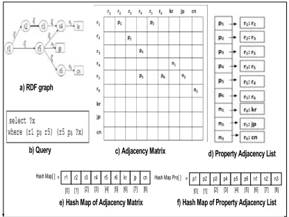
3.2.3 Using Property Adj. Lists with Adj. Matrix First, Adjacency Matrix is used makes aware that it wastes space in case we have sparse graph and suggests for the Adjacency Lists, which saves space but increases the Time Complexity. In case of Adjacency Matrix, two Adjacency Matrices have been used, one for resources and one for property. The Property Adjacency Matrix take lot of space and many of its cells are not used, as for a given property there can’t be much resources add. Hence, it’s not good approach to use Adjacency Matrix. As a solution we can use Adjacency List for property along with Adjacency Matrix approach. Taking the example graph and its equivalent Adjacency Matrix, instead of creating the Adjacency Matrix of properties an Adjacency List can be created as shown in Figure 15. The Figure 17 shows the scenario all together.

p1 p2 p3 p4 p5 p6 n1 n2 n3 [0] [1] [2] [3] [4] [5] [6] [7] [8] =

Hash Map Pro[ ] r1 r2 r3 r4 r5 r6 kr jp cn [0] [1] [2] [3] [4] [5] [6] [7] [8] =

Hash Map[ ]

a) RDF graph

b) Query c) Adjacency Matrix _{d) Property Adjacency List}

e) Hash Map of Adjacency Matrix f) Hash Map of Property Adjacency List

Figure 17: Adjacency Matrix with Adjacency List

Now the query can be answered by increasing a Time Complexity little bit by saving lots of space. The Algorithm to answer the query is given in the Figure 18. Firstly, the subject, property and object are extracted from Triple. Then for whole triples (having subject, property & object known) of query, the Adjacency Matrix is searched out to check either query triple matched graph triple or not. When such

triple extracted that is having missing object, the Algorithm search it in the Adjacency List of Property. Here one more for loop is needed, which iterates the number of object’s or subject’s times that are connected with the property (not very long for loop). The Time Complexity of this Algorithm is also O(m×l), where m is the number of triples in query and l is the number of objects adjacent to the property. But as compared to Adjacency List there is no first for loop is need for each of the triple to find that either the triple exists in the RDF Graph or not, it will find this in constant time O(1).

Figure 18: Algorithm

3.3 Creating Adjacency Matrix directly from Triples

The Adjacency Matrix can be created directly from the Triples. There is no need for Graph representation of the RDF data (made up of number of Triples). Instead of creating Graph first and then creating Adjacency Matrix or list, we can directly create the Adjacency Matrix of the RDF data. This will save lots of space; almost half of the one discussed in previous section.

7606

Figure 19: Example RDF data

Now create Adjacency Matrix by taking subjects on the row side and objects on the column side and filling it with the property between subject and object. The Adjacency Matrix of the Example RDF data in the Figure 19 is shown in the Figure 20. The roughly estimated Space Complexity of the Adjacency Matrix is 15 cells (rows = 3 and columns = 5, hence 5 × 3 = 15). For clarity purpose, the cells have been kept vacant that have no property instead of filling it with zeros.

Figure 20: Adjacency Matrix of RDF data

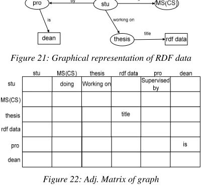
If the Graph representation of RDF data is taken and made its Adjacency Matrix then it will take more space. This can be better understood diagrammatically. The graph representation of the RDF data in the Figure 19 is shown in the Figure 21. Now when storing this graph in Adjacency Matrix more space will be used which measured in cells will be 36 (rows = 6 and columns = 6, hence 6 × 6 = 36).

Figure 21: Graphical representation of RDF data

Figure 22: Adj. Matrix of graph

Hence, it can be concluded that lots of space can be reduced if the Adjacency Matrix will be created directly from the triples. If we first convert RDF data into graph and then produce Adjacency Matrix of graph it will wasted lots of space as many of the subjects and objects will be repeated for none.

The Algorithm used to create Adjacency Matrix from RDF data has been shown in the Figure 23. It first extracts all distinct subjects and objects and then declares Adjacency Matrix of number of distinct subjects and objects. It then populates the matrix by traversing all the triples of RDF data.

Figure 23: Algorithm for creating Adjacency Matrix

In the Adjacency Matrix now it is apparent that there are different subjects and different objects at the dimensions of the Adjacency Matrix. Therefore, there is need of two Hash tables (separately for subjects and Objects). The two Hash Tables for subjects and objects are shown in the Figure 24 and 25.

Figure 24: Hash Table for Subjects

Figure 25: Hash Table for Objects

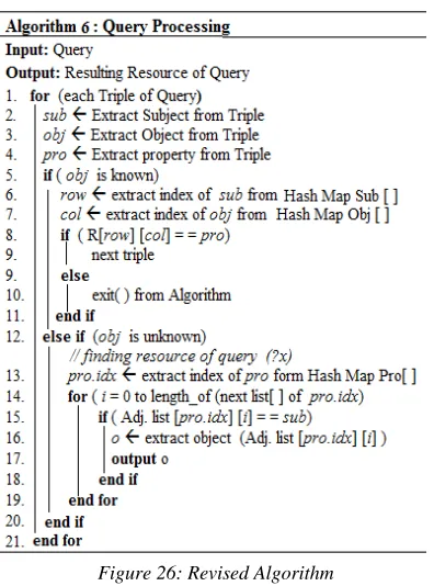
Now, a slight change needs to be made in the Algorithm 5 in the lines # 6 and 7. As separate Hash Tables for Subjects and Objects have been created, therefore the index from these arrays can be created. The new Algorithm is shown in the Figure 26. When the Query will be posed, the indices of the subjects and objects will be extracted from the Hash Map Sub [ ] and Hash Map Obj [ ] and then will be searched in the Adjacency Matrix.

7607 object in the next list of the subject in Master Adjacency List.

Figure 26: Revised Algorithm

3.4.1 Handling Backward Path Queries

The query as shown in the Figure 3 is a Forward Path Query, firstly the triples are given and at the last triple the object is unknown. There are also Backward Path Queries, in which at the start the subject is not given. The one of the examples of such Query is given in the Figure 27. In this query, in the first triple the subject is unknown and subject is to be found out which has a path in forward direction (given in the next triples of where clause). All resources (subjects) are to be found out that precede the path pattern given in a query. The sequence of triples made up the path pattern. To answer the Backward Path Queries we have develop another Algorithm as shown in the Figure 28.

Figure 27: Backward Path Query

It is same as the Algorithm for Forward path query (Figure 28) except the second part of Algorithm. In the second part when the subject of the triple is not known, the algorithm checks in the Property Adjacency List. It first extracts the object of the query triple and searches it in the next adj. list of property. Where the object is matched against that object it extracts the subject. That extracted subject is the desired answer of the query. As shown in the

Query (given in Figure 27), the first triple has missing subject. This subject is found by this Algorithm.

Figure 28: Algorithm for Backward Query using Adjacency Matrix

If the data is dense, means for subjects and objects there are many properties then the data will be stored in form of Adjacency Matrix and will use the Algorithm 6. But if the data is sparse, then using Adjacency Matrix lots of space would be wasted and data is to be stored in Adjacency List. To answer the query when data is stored in Adjacency List then the new algorithm would be needed that is given in the Figure 29. It works same as the above algorithm the only difference is in the first part. The complete triples are searched in the Adjacency lists and when there came any triple with missing subject then the second part would be used to search for the relevant subject. The Time Complexity of both algorithms is same discussed earlier.

3.5 Discussion

7608 there can be high number of properties between the subjects and objects and hence, many of the cells will be filled and there will be very less cells having ‘0’. Therefore, it will be good option to use the Adjacency Matrix instead of Adjacency List. As in this case the Adjacency List will take space almost equal to the Adjacency Matrix (Space Complexity becomes high) and having low efficiency. Hence, Adjacency Matrix will suit more than the Adjacency List. But when the graph is sparse i.e. there are very less properties between subjects and objects then the Adjacency Matrix will waste space and Adjacency List as storage mechanism will suit more.

Figure 29: Algorithm Backward Query using Adjacency Lists

In both cases either the Adjacency Matrix or the Adjacency List, the Property Adjacency Lists has been used because if store it in Adjacency Matrix then it will waste lot of space as there are always not very much nodes connected with properties in both situations (dense or sparse graphs). In many of the situations the some of the properties can have same objects and same subject then it will not be possible both and one will be over write. Hence in both

storing methods the Property Adjacency List would be used.

Secondly, by using a new method to create the Adjacency Matrix a lot of the space can be saved. In RDF Graph the subjects and objects have properties which can be considered and only the subjects and objects which have the properties need to be used to create the Adjacency Matrix not the whole of the subjects and objects need to be considers in each dimension of the Matrix.

4. RESULTS AND DISCUSSION

In this section, various example case studies are taken to investigate the performance of proposed scheme.

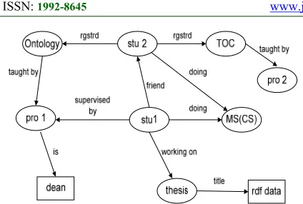
4.1 Example 1

Consider Example RDF data at the Figure 30. The graphical representation of this data as shown in Figure 31 is sparse and the number of properties between nodes is not very high.

4.1.1 Storing the RDF data using Adjacency Matrix

Now, to store this data, we have used both techniques Adjacency Matrix and Adjacency Lists (as proposed). Firstly, the data is stored in Adjacency Matrix directly from the RDF data instead of its graphical representation. We created Adjacency Matrix by using Algorithm at Figure 23 which is shown in the Figure 32. Firstly, all the distinct subjects and objects are extracted from the RDF data (Figure 30) are shown in the Figure 32. We have created hashing over the subjects and Objects such that they can be stored in the Adjacency Matrix according to indices of Hash Tables. The Adjacency Matrix is created by taking subject at row side and objects at column side (shown at Figure 33).

7609

Figure 31: Graphical Representation of Example 1

Figure 32: Extracted Subjects and Objects from Example RDF data 1

Figure 33: Adjacency Matrix of Example 1

The subjects and objects are stored according to indices of Hash Table. We can see that for example ‘stu 1’ has index ‘[0]’ in the Hash Map Sub [] and in the Adjacency Matrix it is put on the same index. We did this to retrieve the indices of subject and object (of Triple) in constant time. After storing data, to answer the query, we also need Adjacency List of properties. The Adjacency List of properties is created by extracting all the properties first then put its adjacent subjects and objects against these properties shown in Figure 35. After extracting the properties, we also produce has Hash Table of it as shown in Figure 34.

Figure 34: Extracted Properties of Example 1

The properties are hashed so that we can find the relevant property quickly (in constant time). When the property in the Query need to be matched with RDF data it will first be searched in the Hash Map

Pro[ ], and the index of property will be return that will point us to the property in the Adjacency List of Property. As we have created the Adjacency List of properties according to the indices in the Hash Map Pro[ ].

Figure 35: Adjacency List of properties

4.1.2 Query Processing

The data is stored now and we should run the query. For this purpose, we have taken an example query which is shown in Figure 36. This is a Forward Path Query in which the whole triples are given first then and a triple with missing object is given. The result of the Query is the missing object which is found out by implanting our algorithm at Figure 26 (Algorithm 6). According to our algorithm, we will extract all the triples one by one. For the whole triples of query, we will match these triples with triples of RDF data stored in Adjacency Matrix. When a triple with missing ‘object’ comes, we will use then Adjacency List of properties to find out the relevant object.

Figure 36: Query 1

When the Algorithm 6 (Figure 28) starts for the query, it first extract triple (line # 1) of Query. According to the Query, the triple will be,

(<stu 2> <regstrd> <Ontology>)

The subject, object and predicate or property will be extract next and stored for further processing (line # 2 to 4).

sub  stu 2, pro  regstrd & obj  Ontology

7610

row  1

col  5

These indices gave us the location of triple in the RDF data. We will switch to the location R [1][5] (R is the name of the Adjacency Matrix of RDF data) and against that cell the property will be matched with the property of the Query (line # 8). If it matched, we will extract next triple of query to be matched. If it will not match we will exit Algorithm as there is no use to search further. When the triple extracted with unknown Object the second part (else if) of the Algorithm will be run. It is used to find the desired Object. In this case, Query with missing object is:

(<pro 1> <is> <?x> )

subpro 1, pro is & obj ?x

Now, instead of Adjacency Matrix the Adjacency List of Properties will be searched. The index of the property of Query will be extracted (line # 13) and tells where will be that property in the Adjacency List.

pro.idx 4

It will tell us the location of the property in the Adjacency Master List. Now, in the next list of property we will search the subject and against that subject extract the Object that will be the answer for the Query. The answer to the Query is ‘dean’.

<stu1> <regstrd> <Ontology> <Ontology> <taught by> <pro1> <pro 1> <is>

<dean>

We have handled the Backward Path Queries too in our proposed work. It will be processed same as the Forward Path Query, with a single difference that now the subject will be extracted. One of the Backward Path Query is given in the Figure 37. For whole triples, it will search in Adjacency Matrix and for the triple with missing ‘subject’ it will search in Adjacency List of properties in a way that it will extract the property of the triple. For that property, in the Property Adjacency List search object which will match with the object of RDF data and extract ‘subject’ against that object.

Figure 37: Query 2

4.1.3 Storing the RDF data using Adjacency List

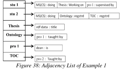
The other technique of storing data is using Adjacency List. Hence, we have also stored the same data in Adjacency List as shown in Figure 38.

The same queries will also run on this data structure also and produce results. To store data, firstly all the subjects will be extracted from the RDF data and Hash table will be created as shown in the Figure 32(a). According to this the Master Adjacency List will be created. Then the adjacent Objects (with their property) to each subject, will stored in the next list of that subject.

Figure 38: Adjacency List of Example 1

4.1.4 Query Processing

The Algorithm 5 at Figure 18 will be used to answer query when data is stored in Adjacency List. We have taken the Query 1 (Figure 36) as an example. The Algorithm is same as the Algorithm 6, with only difference is in the first part of Algorithm in which the Adjacency List is use instead of Adjacency Matrix. The whole triples will now be searched in Adjacency List. In Adjacency List, it will search firstly in Master Adjacency List and then its next lists. For this there a for loop is needed which will decrease the efficiency little. For the missing triple, it will search in the same manner as it is being done Adjacency Matrix’s method.

4.1.5 Comparison of both methods

As the data which have taken as an example is sparse in nature, therefore, the later technique (storing data using Adjacency List) will be preferable in a sense that using Adjacency Matrix wastes a lot of space. This can aptly be seen in the Figure 33. Most of the cells are not utilized because there are very less properties between the subjects and objects. By using Adjacency List, we can save a lot of space but with a little compromise of time efficiency.

4.2 Example No. 2

We have taken such type of data in example 2 of case studies (whose graphical representation is dense). The example data is shown in Figure 39.

When this data is represented through graph, it can evidently be seen that it is a dense graph as shown in Figure 40.

7611 objects, produce their Hash Tables (as shown in Figure 41 (b) & (c)) and then produce Adjacency Matrix of it.

Figure 39: Example RDF data 2

Figure 40: Graphical representation of Example data 2

Figure 41: Storage of Example 2

To answer the missing part of query, the Adjacency List of properties (for both storage methods) has been created and shown in Figure 43(a). The Hash Table for properties has been shown in Figure 42(b). It will be used to produce Master Adjacency List.

After analyzing the comparison between both storage methods, it can explicitly be viewed that in this case Adjacency Matrix is more efficient than Adjacency List considering the both aspects of Time and Space complexities.

Figure 42: Storing Properties

In Figures 44 and 45, the Forward and Backward Path Queries have been shown. Both queries can be answered by both techniques (storing either through Adjacency Matrix or through Adjacency List).

Figure 43: Adjacency List of Example 2

Figure 44: Query 3

The efficiency of algorithms (Figures 25 & 26) is evidently more executable in Adjacency Matrix rather than in Adjacency List.

7612 Considering the above discussed case studies, it can be concluded that when we have a data, we will check the nature of the data and then store it accordingly.

4.3 Example No. 3

Now, we have taken as an example from the one of the research papers (Kim, Sept. 2009) of our Literature Review as shown in Figure 46. This is a graphical representation of RDF data.

Figure 46: Graphical Representation of data

In the proposed technique we used RDF data to produce Adjacency Matrix. Here from the graph we produce the RDF data of our own as shown in the Figure 47. Now we will follow all the steps of our technique to find the result of the Query of that research paper. For the clarity purpose, we have numbered the properties.

Figure 47: RDF data Example 3

4.3.1 Storing the RDF data using Adjacency Matrix

Now, we will store this data in Adjacency Matrix using Algorithm at Figure 33. First, we will extract all the distinct subjects and objects from the RDF data (Figure 47) are stored them by creating hashing over the subjects and Objects (shown in the Figure 48). Then, we will create Adjacency Matrix according to indices of Hash Tables and populate it with properties. We have taken the subjects at row side and objects at column side (shown at Figure 49). 4.3.2 Query Processing

The data is stored, now we will query it (Query 5 in Figure 50). By using Algorithm 6 first, we will extract all the triples of query one by one. For the complete triples of query, we will match these triples with triples of RDF data stored in Adjacency Matrix. As triple with missing ‘object’ extracted, we will use

then Adjacency List of Properties to search out the desired object.

Figure 48: Extracted Subjects and Objects from RDF data Example 3

Figure 49: Adjacency Matrix of Example RDF data 3

Figure 50: Query 5

Algorithm first extract first triple (line # 1) of Query, which is

(< r1 > < p3 > < r5 >)

The subject, object and predicate or property of the corresponding triple will be extracted next and stored (line # 2-4).

sub  r1 , pro  p3 & obj  r5

Now the Object of the Triple (as above) will be checked (line # 5) either it is known or not. As it is known, now we will check either this Query Triple exists in the RDF data or not. We then extract the indices of subject and object (from Hash Map Sub[ ] & Hash Map Obj[ ] respectively) and use these indices for Adjacency Matrix (line # 6 & 7).

row  0 col  3

Now check for the location R [0][3] (R is the Adjacency Matrix of RDF data) the property. If matched with the property of the Query Triple (line # 8). If not matched we will exit Algorithm without proceeding further. When such triple extracted having Object unknown the second part (else if) of the Algorithm will be executed. This part is used to find the unknown Object. Here the Query Triple with missing object is as below.

7613 sub  r5, pro  p6 & obj  ?x

Now, instead of Adjacency Matrix the Adjacency List of Properties will be used to find the missing ‘Object’. The index of the property of Query Triple will be extracted (line # 13) from the Hash Map Pro[] (Figure 51) and tells about the property in the Adjacency List of Properties (Figure 52).

pro.idx  4

Figure 51: Hash Map of Properties

This index will tell us the location of the property in the Master List of Adjacency List. Now, in the next list[ ] of this property we will search the subject and for this subject extract the Object that is will be the result of the Query. The result of the Query 5 is ‘r6’.

(< r1 > < p3 > < r5 >) (< r5 > < p6 > < r6 >) Consider the Backward Path given in the Figure 53. It will be processed same like Forward Path Query, with one difference that now the subject will be searched out. The Algorithm at the Figure 39 will be used to find the missing ‘Subject’ of the Query 6. For complete triples, it will search in Adjacency Matrix for the triple with missing ‘subject’ it will search in Adjacency List of properties in a way that it will extract the property of the triple. For that property, in the Property Adjacency List searched for given object in triple of query, which will be matched with the object of RDF data and if found against that object extract ‘subject’.

Figure 52: Adjacency List of Properties

Figure 53: Query 6

4.3.3 Storing the RDF data using Adjacency List Now we will store the same data using Adjacency List as shown in Figure 54. Same queries will also run on this data structure also and produce results.

Figure 54: Adjacency List of Example 3

4.3.4 Query Processing

The Algorithm 5 will be used for answering the query, when data is stored in Adjacency List. We have taken the Query 5 as an example. The Algorithm is same as the Algorithm 6, with only one difference in first part of Algorithm. In the First part of Algorithm 5 the Adjacency List is use instead of Adjacency Matrix. The whole triples will now be searched in Adjacency List. For searching in Adjacency List, it will be first searched Master Adjacency List and then its next lists. Hence, due to this there is a for loop used, which will decrease the efficiency (but little). For the triple with missing Object, it will search in the same manner as it is being done in Adjacency Matrix Algorithm (using Adjacency List of Properties). It can be seen that as the data is sparse, the Adjacency Lists fits more to store data.

5. CONCLUSION

7614 Consequently, two storage mechanisms were proposed. If the data is dense then Adjacency Matrix was suggested and in case of sparse data Adjacency Matrix was suggested to store RDF data. Then based on the storage of RDF data Algorithms are devised. Moreover, an improved method to store RDF data in Adjacency Matrix directly from the triples is proposed. Finally, the case studies are presented to show the effectiveness of the proposed techniques and comparison with other state of the art techniques is given. In future, further optimization will be investigated in contrast to various query optimization techniques.

REFERENCES

[1]. Y. Yan, C. W. A. Z. W. Q. L. M. a. Y. P., 2009. Efficient Indices using Graph Partitioning in RDF. s.l., s.n.

[2]. Akiyoshi Matono, T. A. M. Y. S. U., 2005. A Path-based Relational RDF Database. s.l., The 16th Australasian Database Confrence. [3]. Shady Elbassuoni, R. B., 2011. Keywords

search over RDF data. Scotland, UK., s.n. [4]. Baolin Lui, B. H., 2010. HPRD: A High

Performance RDF Database. International Journal of Parallel, Emergent and Distributed Systems, Volume 25.

[5]. Matono, e. a., Sept. 2003. An Indexing Scheme for RDF and RDF Schema based on Suffix Arrays. s.l., First International Workshop on Semantic Web and Databases (SWDB). [6]. Kim, S. W., Sept. 2009. Improved Processing

of Path Query on RDF Data Using Suffix Array. Journal of Convergence Information Technology, Volume 4.

[7]. Y. Yan, C. W. A. Z. W. Q. L. M. a. Y. P., 2008. “Efficiently querying rdf data in triple stores, Beijing, China.: s.n.

[8]. Anon., 2013. SPARQL Query Laguage for RDF. [Online]http://www.w3.org/TR/rdf-sparql-query

[9]. Hutt, K., 2005. A Comparison of RDF Query Languages. 21st Computer Science Seminar. [10]. Manber, U. M. E., 1993. Suffix Arrays: A New

Method for On-Line String Searches. SIAM. J. on Computing, p. 935–948.

[11]. Morin, P., 2012. Open Data Structures. Edition 0.1E ed. s.l.:s.n.

[12]. David C. FAYE, O. C. ,. G. B., 2012. A survey of RDF storage approaches. ARIMA Journal, Volume vol. 15.

[13]. Seaborne, A., 2004. “RDQL, A Query Language for RDF". [Online] Available at: http://www.w3.org/submission/2004/subm-rdql

[14]. Anon., 2012. Minimal Perfect Hash Functions - Introduction. [Online] Available at: http://cmph.sourceforge.net/concepts.html [15]. Anon., 2013 . SPARQL. [Online] Available at:

http://en.wikipedia.org/wiki/SPARQL [16]. Anon., 2000. RDF schema. [Online] Available

at: http://www.w3.org/TR/2000/CR-rdf-schema-20000327/

[17]. Anon., 2013. http://www.foaf-project.org/. [Online]

[18]. Anon., 2013. Triple store. [Online] Available at: http://en.wikipedia.org/wiki/Triplestore/ [19]. Abadi, D. J. M. A. M. S. R. a. H. K., 2009.

SW-Store: A Vertically Partitioned DBMS for Semantic Web Data Management. VLDB Journal.