Image compression and reconstruction using modified fast Haar wavelet transform

IMAGE COMPRESSION AND RECONSTRUCTION USING

MODIFIED FAST HAAR WAVELET TRANSFORM

Soni P.

Department of ECE Sahrdaya College of Engineering &Technology Thrissur, Kerala, India E-Mail: [email protected]

ABSTRACT

Image compression is minimizing the size of a graphics file keeping the quality of the image to an acceptable level. Wavelets are mathematical tools for hierarchically decomposing functions. It allows to describe a function in terms of a coarse overall shape, plus details that range from broad to narrow. Haar Transform lends itself easily to simple manual calculations. Modified Fast Haar Wavelet Transform (MFHWT), is one of the algorithms which can reduce the calculation work in Haar Transform (HT) and Fast Haar Transform (FHT). The project is an attempt on implementation of an efficient algorithm for compression and reconstruction of images, using MFHWT.

Keywords: image compression, wavelet transform, haar transform, FHT, quantization, sub band coding, MFHWT.

INTRODUCTION

Image compression plays a vital role in applications like video conferencing, remote sensing, medical imaging, magnetic resonance imaging etc. In most images the neighboring pixels are correlated and hold redundant information. The task then is to find out less correlated representation of the image. Two elementary components of compression are redundancy and irrelevancy reduction. Redundancy reduction aims at removing duplication from the signal source image. Irrelevancy reduction omits parts of the signal that is not noticed by the signal receiver.. Number of bits required to represent the information in an image can be minimized by removing the redundancy present in it. There are three types of redundancies: spatial redundancy, which is due to the correlation or dependence between neighboring pixel values; spectral redundancy, which is due to the correlation between different color planes or spectral bands; temporal redundancy, which is present because of correlation between different frames in images.

Image compression aims to reduce the number of bits required to represent an image by removing the spatial and spectral redundancies as much as possible. If n1 and n2 denote the number of information carrying units in original and compressed image respectively, then the compression ratio CR can be defined as CR=n1/n2; And relative data redundancy RD of the original image can be defined as RD=1 - 1/CR;

Figure-1. Image Compression model.

Figure-2. Image decompression model.

A transformer transforms the input data into a format to reduce inter-pixel redundancies in the input image. Transform coding techniques use a reversible, linear mathematical transform to map the pixel values onto a set of coefficients, which are then quantized and encoded. Many of the resulting coefficients for most natural images have small magnitudes and can be quantized without causing significant distortion in the decoded image. The higher the capability of compressing information in fewer coefficients, the better the transform; so, the Discrete Cosine Transform (DCT) and Discrete Wavelet Transform (DWT) have become the most widely used transform coding techniques. Transform coding algorithms usually start by calculating transform coefficients , effectively converting the original pixel values into an array of coefficients within which the coefficients closer to the top-left corner usually contain most of the information needed to quantize and encode the image with little perceptual distortion. The resulting coefficients are then quantized and the output of the quantizer is used by symbol encoding techniques to produce the output bitstream representing the encoded image. In image decompression model at the decoder’s side, the reverse process takes place. But the dequantization stage will only generate an approximated version of the original coefficient values.

The zig-zag scanning pattern for run-length coding of the quantized DCT coefficients was established in the original MPEG standard. The same pattern is used for luminance and for chrominance.

Symbol (entropy) encoder creates a fixed or variable-length code to represent the quantizer’s output and maps the output in accordance with the code. It compresses the compressed values obtained by the quantizer to provide more efficient compression. Most important types of entropy encoders used in lossy image compression techniques are arithmetic encoder, Huffman encoder and run-length encoder. For applications requiring fast execution, simple Run Length Encoding (RLE) is very effective.RLE is a very simple form of data compression in which runs of data are stored as a single data value and count. Each time a long run is encountered in the input data, two values are written to the output file. The first of these values is the character itself, i.e., a flag to indicate that run-length compression is beginning. The second value is the number of characters in the run.

WAVELET TRANSFORM

An image can be well-approximated by a sparse set of clustered significant coefficients in wavelet domain, and intelligent coding tools can be designed to reduce the bit rate required for coding this set. Wavelet transform exploits both the spatial and frequency correlation of data by dilations (or contractions) and translations of mother wavelet on the input data. It supports the multi resolution analysis of data, which allows progressive transmission and zooming of the image without the need of extra storage. It is also symmetric. That is both the forward and the inverse transform has the same complexity, building fast compression and decompression routines.

The implementation of wavelet compression scheme is very similar to that of sub band coding scheme: the signal is decomposed using filter banks. Filters of different cut-off frequencies analyse the signal at different scales. The output of the filter banks is down-sampled, quantized, and encoded. The decoder decodes the coded representation, up-samples and recomposes the signal. If a signal is put through two filters:

(i) a high-pass filter, high frequency information is kept, low frequency information is lost.

(ii) a low pass filter, low frequency information is kept, high frequency information is lost.

then the signal is effectively decomposed into two parts, a detailed part (high frequency), and an approximation part (low frequency).

The sub signal produced from the low filter will have a highest frequency equal to half that of the original. According to Nyquist sampling this change in frequency range means that only half of the original samples need to be kept in order to perfectly reconstruct the signal. So, up-sampling can be used to remove every second sample. The approximation sub signal can then be put through a filter bank, and this is repeated until the required level of decomposition has been reached.

The DWT is obtained by collecting together the coefficients of the final approximation sub signal and all the detail sub signals. If all the details are ’added’ together then the original signal should be reproduced. The ideas are shown in the figure below.

Figure-3. Filter banks.

Figure-4. Sub-band coding example.

The approximation subsignal shows the general trend of pixel values and other three detail subsignals show the vertical, horizontal and diagonal details or changes in the images. If these details are very small (threshold) then they can be set to zero without significantly changing the image

Conservation and Compaction of Energy

Energy is defined as the sum of the squares of the values. So the energy of an image is the sum of the squares of the pixel values. The energy in the wavelet transform of an image is the sum of the squares of the transform coefficients. During wavelet analysis the energy of a signal is divided between approximation and details signals but the total energy does not change. During compression however, energy is lost because thresholding changes the coefficient values and hence the compressed version contains less energy. The compaction of energy describes how much energy has been compacted into the approximation signal during wavelet analysis. Compaction will occur wherever the magnitudes of the detail coefficients are significantly smaller than those of the approximation coefficients. Compaction is important when compressing signals because the more energy that has been compacted into the approximation signal the less energy can be lost during compression. If the energy retained (amount of information retained by an image after compression and decompression) is 100% then the compression is lossless as the image can be reconstructed exactly. This occurs when the threshold value is set to zero, meaning that the details have not been changed. If any value is changed then energy will be lost and thus lossy compression occurs. As more zeros are obtained, more energy is lost. Therefore, a balance between the two needs to be found out.

Compression Techniques

This investigation will concentrate on transform coding and then more specifically on Wavelet Transforms. Image data can be represented by coefficients of discrete image transforms. Coefficients that make only small contributions to the information contents can be omitted. Usually the image is split into blocks (subimages) of 8x8 or 16x16 pixels, then each block is transformed separately. However this does not take into account any correlation between blocks, and creates "blocking artifacts" . However wavelets transform is applied to entire images, rather than sub images, so it produces no blocking artifacts. This is a major advantage of wavelet compression over other transform compression methods.

How Wavelets Work

The Haar function can be described as a step function ψ (t)

In order to perform wavelet transform, Haar wavelet uses translations and dilations of the function, i.e. the transform make use of following function:

where this is the basic works for wavelet expansion A Haar Transform decomposes each signal into two components, one is called average (approximation) or trend and the other is known as difference (detail) or fluctuation

By taking average and difference from two nodes from previous level, approximate coefficients and detail coefficients for next level, n −1, n − 2, n − 3, of

decomposition nodes are counted. The process is called Fast Haar Transform, FHT.

A precise formula for the values of first average

sub signal, at one level for a

signal of length N i.e. is

and the first detail subsignal,

at the same level is given as

The procedure may be explained with the help of a simple example as shown below. Apply 2D HT to the following finite 2D signal.

using 1D HT along first row, the approximation coefficients are

The same transform is applied to the other rows of I. By arranging the approximation parts of each row transform in the first two columns and the corresponding detail parts in the last two columns we get the following results, in which approximation and detail parts are separated by dots in each row

By applying the following step of 1D HT to the columns of the resultant matrix, we find that the resultant matrix at first level is

Thus we have

Each piece shown in example 1 has a dimension (number of rows/2) × (number of columns /2) and is called A, H, V and D respectively. A (approximation area) includes information about the global properties of analysed image. Removal of spectral coefficients from this area leads to the biggest distortion in original image H. (horizontal area) includes information about the vertical lines hidden in image. Removal of spectral coefficients from this area excludes horizontal details from original image V. (vertical area) contains information about the horizontal lines hidden in image. Removal of spectral coefficients from this area eliminates vertical details from original image D. (diagonal area) embraces information about the diagonal details hidden in image. Removal of spectral coefficients from this area leads to minimum distortions in original image. To get the value at next level, again HT is applied row and column wise on the piece A, obtained earlier as in example 1. Repeating this process recursively on the averages gives the full decomposition. We can reconstruct the image to any resolution by recursively adding and subtracting the detail coefficients from the lower resolution versions. Thus the HT is suitable for application when the image matrix has number of rows and columns as a multiple of 2.

Fast Haar Transform (FHT) involves addition, subtraction and division by 2, due to which it becomes faster and reduces the calculation work in comparison to HT. For the decomposition of an image, we first apply 1D FHT to each row of pixel values of an input image matrix.

These transformed rows are themselves an image and we apply the 1D FHT to each column. The resulting values are all detail coefficients except for a single overall average coefficient. Figure. shows calculation of the typical Fast Haar Transform, FHT, for n = 4 , given by the

data

Generally, the process is called wavelet decomposition and the detail coefficients are normally called as wavelet transform coefficients where these nodes will be considered in threshold process as well as reconstruction works in multi-resolution wavelet. In many applications especially signal processing, threshold wavelet coefficients can be done to clean out “unnecessary” details which are consider as noise. Then, the data can be obtained again through wavelet reconstruction. For the multi-resolution wavelet, the detail coefficients (wavelet transform coefficients) are needed to reconstruction the original data while the approximation coefficients are not necessarily involved. Mathematically, we regard wavelet decomposition (analysis) and reconstruction (synthesis) as wavelet transform and inverse of wavelet transform.

The transformation of the 2D image applies the 1D wavelet transform to each row of pixel values. This operation provides us an average value along with detail coefficients for each row. Next, these transformed rows are treated as if they were themselves an image and apply the 1D transform to each column. The resulting values are all detail coefficients except a single overall average co-efficient. In order to complete the transformation, this process is repeated recursively only on the quadrant containing averages.

The matrix representing this image is shown in Figure.

Now we perform the operation of averaging and differencing to arrive at a new matrix representing the same image in a more concise manner. Consider the first row of the Figure.

Averaging: (64+2)/2=33, (3+61)/2=32, (60+6)/2=33, (7+57)/2=32

Differencing: 64–33 =31, 3–32= –29, 60–33=27 and 7– 32= –25

The transformed row becomes (33 32 33 32 31 –29 27 – 25).

Now the same operation on the average values i.e. (33 32 33 32) is performed. i.e. first two elements of the new transformed row. Thus the final transformed row becomes (32.5 0 0.5 0.5 31 –29 27 –25). The new matrix we get after applying this operation on each row of the entire matrix is shown in Figure.

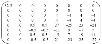
Performing the same operation on each column of the matrix in Figure, we get the final transformed matrix as shown in Figure. This operation on rows followed by columns of the matrix is performed recursively depending on the level of transformation. The left-top element of the Figure. i.e. 32.5 is the only averaging element which is the overall average of all elements of the original matrix and the rest all elements are the details coefficients. The point of the wavelet transform is that regions of little variation in the original image manifest themselves as small or zero elements in the wavelet transformed version. The 0’s in the Figure are due to the occurrences of identical adjacent elements in the original matrix. A matrix with a high proportion of zero entries is said to be sparse. For most of

the image matrices, their corresponding wavelet transformed versions are much sparser than the originals. The original matrix can be easily calculated just by the reverse operation of averaging and differencing i.e. the original image can be reconstructed from the transformed image without the loss of information. Thus, it yields a lossless compression of the image.

Figure-6. Final transformed matrix after one step.

However, to achieve more compression, we have to think of the lossy compression. In this case, a nonnegative threshold value say ∑ is set. Then any detail coefficient in the transformed data whose magnitude is less than or equal to ∑ is set to zero. It will increase the number of 0’s in the transformed matrix and thus the level of compression is increased. So, ∑=0 is used for a lossless compression. If the lossy compression is used, the approximations of the original image can be built up. The different thresholding methods we have used are: hard thresholding, soft thresholding and universal thresholding. These thresholding methods are defined as follows:

where  is the standard deviation of the wavelet coefficients and N is the number of wavelet coefficients.

In this paper, only the gray-scale images are considered. However, wavelet transforms and compression techniques are equally applicable to color images with three color components.

ALGORITHM OF MFHWT IN 2D

A 2D MFHWT can be done by performing the following steps:

- Read the image as a matrix.

- Apply MFHWT, along row and column on entire matrix of the image to get a transformed image matrix of one level of input image.

- For reconstruction process, FHT is used on the image matrix obtained in the above step. Calculate MSE and PSNR for reconstructed image.

At each level in MFHWT we need to store only half of the original data used in FHT. For MFHT, its can be done by just taking (w+ x + y + z)/ 4 instead of (x + y)/

2 for approximation and (w+ x −y −z)/ 4 instead of (x − y)/ 2 for differencing process. 4 nodes have been

considered at one time. The calculation for (w+ x −y −z)/

4 will yield the detail coefficients in the level of n − 2 . For

the purpose of getting detail coefficients, differencing process (x −y)/ 2 still need to be done.

Figure-7. Modified Fast Haar Transform, MFHT.

Compression steps:

-.Digitize the source image into a signal s, which is a string of numbers and read the image as a matrix.

-.Transform the signal into a sequence of wavelet coefficients w

-.Use threshold to modify the wavelet coefficients from w to w’.

-.Zig-zag scanning of the coefficients. - Run length encoding.

- Entropy encoding (optional- if further compression is required)

Reconstruction steps: -Decode the sequence -Reverse the zigzag pattern

-Take Inverse transform of the coefficients.

RESULTS COMPRESSION

Figure-8. Original image (cameraman.tif) compressed

image size 256 * 256 decompression.

Figure-9. Original image reconstructed image (256*256).

CONCLUSION AND FUTURE WORKS

As part of the project, the algorithm was implemented in MATLAB using certain MATLAB functions and C programming language. The results were verified.

Further compression can be achieved by: - changing the threshold value.

- Including an entropy coding method like Huffman coding.

- Can include a BWT block and MTF coding before run length encoding.

The algorithm can be applied for colour images also- RGB matrices would have to be converted into grey scale intensity image.

REFERENCES

[1] Anuj Bhardwaj and Rashid Ali. 2009. “Image Compression Using Modified Fast Haar Wavelet Transform”World Applied Sciences Journal, Vol. 7, No. 5, pp. 647-653, 2009ISSN 1818-4952 © IDOSI Publications.

[2] Phang Chang and Phang Piau. 2007. “Modified Fast and Exact Algorithm for FastHaar Transform”. World Academy of Science, Engineering and Technology, Vol. 35.

[3] “Introduction to Datacompression” by Khalid Sayood.