Uncertainty contributions to low flow projections in Austria

www.hydrol-earth-syst-sci.net/20/2085/2016/ doi:10.5194/hess-20-2085-2016

© Author(s) 2016. CC Attribution 3.0 License.

Uncertainty contributions to low-flow projections in Austria

Juraj Parajka1, Alfred Paul Blaschke1, Günter Blöschl1, Klaus Haslinger2, Gerold Hepp3, Gregor Laaha4, Wolfgang Schöner5, Helene Trautvetter3, Alberto Viglione1, and Matthias Zessner3

1_{Institute for Hydraulic and Water Resources Engineering, TU Wien, Vienna, Austria}

2_{Climate Research Department, Central Institute for Meteorology and Geodynamics, Vienna, Austria} 3_{Institute for Water Quality, Resource and Waste Management, TU Wien, Vienna, Austria}

4_{Institute of Applied Statistics and Computing, University of Natural Resources and Life Sciences (BOKU), Vienna, Austria} 5_{Department of Geography and Regional Science, University of Graz, Graz, Austria}

Correspondence to:J. Parajka ([email protected])

Received: 29 October 2015 – Published in Hydrol. Earth Syst. Sci. Discuss.: 27 November 2015 Revised: 5 April 2016 – Accepted: 12 May 2016 – Published: 26 May 2016

Abstract. The main objective of the paper is to understand the contributions to the uncertainty in low-flow projections resulting from hydrological model uncertainty and climate projection uncertainty. Model uncertainty is quantified by different parameterisations of a conceptual semi-distributed hydrologic model (TUWmodel) using 11 objective functions in three different decades (1976–1986, 1987–1997, 1998– 2008), which allows for disentangling the effect of the ob-jective function-related uncertainty and temporal stability of model parameters. Climate projection uncertainty is quanti-fied by four future climate scenarios (ECHAM5-A1B, A2, B1 and HADCM3-A1B) using a delta change approach. The approach is tested for 262 basins in Austria.

The results indicate that the seasonality of the low-flow regime is an important factor affecting the performance of model calibration in the reference period and the uncertainty ofQ95low-flow projections in the future period. In Austria,

the range of simulatedQ95in the reference period is larger in

basins with a summer low-flow regime than in basins with a winter low-flow regime. The accuracy of simulatedQ95may

result in a range of up to 60 % depending on the decade used for calibration.

The low-flow projections of Q95 show an increase of low

flows in the Alps, typically in the range of 10–30 % and a de-crease in the south-eastern part of Austria mostly in the range

−5 to−20 % for the climate change projected for the future period 2021–2050, relative the reference period 1978–2007. The change in seasonality varies between scenarios, but there is a tendency for earlier low flows in the northern Alps and later low flows in eastern Austria. The total uncertainty of

Q95 projections is the largest in basins with a winter

low-flow regime and, in some basins the range ofQ95projections

exceeds 60 %. In basins with summer low flows, the total un-certainty is mostly less than 20 %. The ANOVA assessment of the relative contribution of the three main variance com-ponents (i.e. climate scenario, decade used for model cali-bration and calicali-bration variant representing different objec-tive function) to the low-flow projection uncertainty shows that in basins with summer low flows climate scenarios con-tribute more than 75 % to the total projection uncertainty. In basins with a winter low-flow regime, the median contribu-tion of climate scenario, decade and objective funccontribu-tion is 29, 13 and 13 %, respectively. The implications of the uncertain-ties identified in this paper for water resource management are discussed.

1 Introduction

assump-tions used in the projecassump-tions translate into uncertainty of es-timated future low flows.

There are numerous regional and national studies that have analysed the effects of climate change on the streamflow regime, including low flows (e.g. Feyen and Dankers, 2009; Prudhomme and Davies, 2009; Chauveau et al., 2013, among others). Most of them apply outputs from different global or regional climate circulation models, which are based on different emission scenarios. The projections of low flows are then typically simulated by hydrologic models of various complexity. There is an increasing number of studies eval-uating different sources of uncertainty in river flow projec-tions resulting from different global climate models (GCMs), downscaling methods or hydrologic model parameterisation (e.g. Dobler et al., 2012; Finger et al., 2012; Coron et al., 2012; Addor et al., 2014; Chiew et al., 2015). Only few stud-ies, however, evaluate the uncertainty of low-flow projections and the relative contribution of its different sources (i.e. cli-mate projection, hydrologic model structure and/or model parameterisations). Such studies include assessment of the impact of different climate projections on low flows evalu-ated, e.g., in Huang et al. (2013) and Forzieri et al. (2014). While Huang et al. (2013) assessed the low-flow changes and uncertainty in the five largest river basins in Germany, Forzieri et al. (2014) evaluated the uncertainty of an ensem-ble of 12 bias corrected climate projections in the whole of Europe. Both studies quantified uncertainty in terms of the number of low-flow projections that suggest the same change direction. Their results indicated a consistent pattern of low-flow changes across different regions in Europe. A common feature of such ensemble climate scenarios is an increase in the agreement between ensemble members with increasing future time horizon of climate projections. The impact of hy-drologic model structure and climate projections was eval-uated in Dams et al. (2015). They applied four hydrologic models calibrated with four objective functions to simulate the impact of three climate projections on low flows for a basin in Belgium. They found that besides the uncertainty introduced by climate change scenarios, hydrologic model selection introduces an additional considerable source of certainty in low-flow projections. The model structure un-certainty was particularly important under more extreme cli-mate change scenarios. A similar study was performed by Najafi et al. (2011), who investigated the uncertainty stem-ming from four hydrologic models calibrated by three ob-jective functions and applied on eight GCM simulations in a basin in Oregon. Their results showed that although in gen-eral the uncertainties from the hydrologic models are smaller than from GCM, in the summer low-flow season the impact of hydrologic model parameterisation on overall uncertainty is considerably larger than that of the GCM.

The quantification of the relative contribution of differ-ent sources to the overall uncertainty of streamflow projec-tions has been recently evaluated by using analyses of vari-ance (ANOVA) (von Storch and Zwiers, 1999). Bosshard

et al. (2013) synthesised previous studies that investigated hydrological climate-impact projections and their sensitivity to different uncertainty sources. They propose an ANOVA framework to separate the uncertainty from climate models, statistical post-processing (bias correction and delta change approach) and hydrological models. Addor et al. (2014) used the ANOVA framework to quantify the uncertainty of stream-flow projections resulting from the combination of emission scenarios, regional climate models, post-processing methods and hydrological models of different complexity. They re-ported that the main source of uncertainty stems from the cli-mate models and natural clicli-mate variability, and the impact of emission scenario increases with increasing future time horizon of climate projections. Hingray and Said (2014) pro-posed a quasi-ergodic two-way ANOVA framework for the partitioning of the total uncertainty of climate projections. This framework has been recently tested for the estimation of climate and hydrological uncertainties of transient low-flow projections in two basins in the southern French Alps (Vidal et al., 2015). The results showed that a large part of the total uncertainty arises from the hydrological modelling and it can be even larger than the contribution from the GCMs.

The objective of this paper is to understand the relative contribution of the impact of hydrologic model calibration and ensemble climate scenarios to the overall uncertainty of low-flow projections in Austria. Here, the uncertainty and variability of low-flow projections is assessed for four climate scenarios, 11 variants of objective functions and 3 decades used for model calibration. Austria is chosen as a case study since it is an ideal test bed for such analysis, as it allows one to disentangle the uncertainties separately in regions with summer and winter low-flow regimes. The as-sessment of uncertainties for winter and summer low-flow regimes allows one to make generalisation for a similar spec-trum of physiographic conditions around the world.

2 Methodology

2.1 Low-flow projections

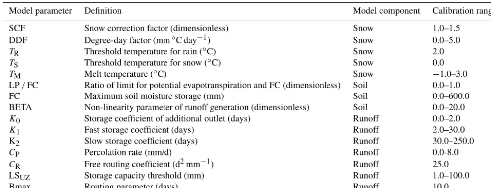
Table 1.TUWmodel parameters. Calibration range is given for parameters calibrated by an automatic routine. Parameters with fixed value are not calibrated.

Model parameter Definition Model component Calibration range

SCF Snow correction factor (dimensionless) Snow 1.0–1.5

DDF Degree-day factor (mm◦C day−1) Snow 0.0–5.0

TR Threshold temperature for rain (◦C) Snow 2.0

TS Threshold temperature for snow (◦C) Snow 0.0

TM Melt temperature (◦C) Snow −1.0–3.0

LP/FC Ratio of limit for potential evapotranspiration and FC (dimensionless) Soil 0.0–1.0

FC Maximum soil moisture storage (mm) Soil 0.0–600.0

BETA Non-linearity parameter of runoff generation (dimensionless) Soil 0.0–20.0

K0 Storage coefficient of additional outlet (days) Runoff 0.0–2.0

K1 Fast storage coefficient (days) Runoff 2.0–30.0

K2 Slow storage coefficient (days) Runoff 30.0–250.0

CP Percolation rate (mm/d) Runoff 0.0-8.0

CR Free routing coefficient (d2mm−1) Runoff 25.0

LSUZ Storage capacity threshold (mm) Runoff 1.0–100.0

Bmax Routing parameter (days) Runoff 10.0

monthly delta changes, with no change in the frequency of rainy days. The daily air temperature is changed by the abso-lute value of monthly delta changes. The differences between daily simulations of a hydrologic model in the reference and future periods are then used to interpret potential impacts of changing climate on future river flows.

The future low-flow changes are quantified by the Q95

low-flow quantile and seasonality index (SI). TheQ95

rep-resents river flow that is exceeded on 95 % of the days of the entire reference or future period. This characteristic is one of the low-flow reference characteristic, which is widely used in Europe (Laaha and Blöschl, 2006). SI represents the average timing of low flows within a year (Laaha and Blöschl, 2006, 2007). It is estimated from the Julian dates Dj of all days when river flows are equal or belowQ95in the reference or

future periods.Dj represents a cyclic variable. Its directional angle, in radians, is given by

θj=

Dj·2π

365 . (1)

The arithmetic mean of Cartesian coordinatesxθandyθof a total ofnsingle daysj is defined as

xθ= 1

n X

j

cos(θj)

yθ= 1

n X

j

sin(θj). (2)

From this, the directional angle of the mean vector may be calculated by

θ=arctan

_y

θ

xθ

1st and 4th quadrant:x >0, (3)

θ=arctan

_y

θ

xθ

+π 2nd and 3rd quadrant:x <0. (4)

Finally, the mean day of occurrence is obtained from re-transformation to Julian date:

SI=θ·365

2π (5)

and the variability of the date of occurrence about the mean date (i.e. seasonality strength) is characterised by the length parameterr. The parameterris estimated as (Burn, 1997)

r=

p

¯

x2_{+ ¯y}2

n (6)

and ranges from r=0 (low strength, uniform distribution around the year) to r=1 (maximum strength, all extreme events of low flows occur on the same day).

The SI is estimated for observed and simulated low flows. The differences between model simulations (i.e.Q95and SI

estimates) in the reference and future periods are then used to quantify potential impacts of climate change on low flows. BothQ95and SI measurements are estimated independently

for the reference and future periods by the lfstat package in R software (Koffler and Laaha, 2014).

2.2 Hydrologic model

In this study, the TUWmodel is calibrated by using the SCE-UA (Shuffled Complex Evolution) automatic calibra-tion procedure (Duan et al., 1992). The objective funccalibra-tion (ZQ) used in calibration is selected on the basis of prior anal-yses performed in different calibration studies in the study re-gion (see e.g. Parajka and Blöschl, 2008; Merz et al., 2011). It consists of the weighted average of two variants of Nash– Sutcliffe model efficiency,MEandM_Elog. While theME

effi-ciency emphasise the high flows, theM_Elogefficiency accen-tuates more the low flows. The maximised objective function

ZQis defined as

ZQ=wQ·ME+(1−wQ)·MElog, (7)

wherewQrepresents the weight on high or low flows. IfwQ equals 1 then the model is calibrated to high flows, if it equals 0 then to low flows only.MEandM

log

E are estimated as

ME=1−

n

P

i=1

Qobs,i−Qsim,i

2

n

P

i=1

Qobs,i−Qobs 2

, (8)

M_Elog=1− n

P

i=1

log(Qobs,i)−log(Qsim,i)

2

n

P

i=1

log(Qobs,i)−log(Qobs

2 , (9)

whereQsim,i is the simulated discharge on dayi,Qobs,i is the observed discharge,Qobsis the average of the observed

discharge over the calibration (or verification) period of n

days.

2.3 Uncertainty estimation

The uncertainty, defined as the range of simulated low-flow indices, is evaluated for two contributions. The first analy-ses the uncertainty (i.e. the range ofQ95 and SI) estimated

for different variants of hydrologic model calibration. Here, two cases are evaluated. In order to assess the impact of time stability of model parameters (Merz et al., 2011), the TUWmodel is calibrated separately for 3 different decades (1976–1986, 1987–1997, 1998–2008). The effect of objec-tive functions used for the TUWmodel calibration is evalu-ated by comparing 11 variants of weights (wQ) used inZQ. The followingwQare tested: 0.0, 0.1, 0.2, 0.3, 0.4, 0.5, 0.6, 0.7, 0.8, 0.9 and 1.0. The hydrologic model is calibrated for all 11 variants in each selected decade. Calibrated models are then used for flow simulations and henceQ95and SI

estima-tion in the reference and future periods.

The second contribution evaluates the uncertainty ofQ95

and SI changes simulated for different climate scenarios. The effect of calibration uncertainty (case 1) is compared for four selected climate scenarios (more details are given in Sect. 3). The delta change approach is used to derive model forcing

for selected future period and simulated future river flows are compared to model simulations in the reference period 1976–2008. The relative changes ofQ95 and SI values

be-tween reference and future periods are estimated for 4 se-lected climate scenarios, 11 variants of model calibration and 3 selected decades. The relative contribution of the impact of model calibration (i.e. time stability and objective function selection) and climate scenario is evaluated for two low-flow regimes and for individual stations over Austria.

The uncertainty of low-flow projections is then compared to the range of low-flow indices obtained by different cali-bration variants in the reference period. In addition, the to-tal uncertainty of future low-flow projections is decomposed to individual components by means of analysis of variance (ANOVA; e.g. von Storch and Zwiers, 1999, chap. 9 for a general introduction to ANOVA). The three-way ANOVA approach is employed to decompose total uncertainty of the projected low-flow changes into three main variance compo-nents. These variance components represent uncertainty con-tributions of three main effects: climate scenario (factor A withI=4 levels), decade used for model calibration (fac-tor B withJ=3, levels) and calibration variant representing different objective functions (factorC withK=11 levels). The ANOVA model is defined as follows:

1Q95ij k=µ+αi+βj+γk+ij k. (10)

In this linear equation (Eq. 10), 1Q95ij k denotes the en-semble projected changes inQ95for the future horizon at a

gauge. It is modelled by a global meanµand the mean effects (deviations of factor-means from the global mean) of climate scenario (αi;i=1, . . ., I ), decade (βj;j=1, . . ., J )and cal-ibration variant (γk;k=1, . . ., K), and ij k are the residual errors of the model. In an ANOVA framework, the total vari-ance of1Q95ij kis characterised by the total sum of squares SST, and is decomposed into additive variance components of individual effects:

ST=SSA+SSB+SSC+SSE. (11)

The variance components of the main effects A, B and C are computed as follows:

SSA=J K

I

X

i=1

(y¯i..− ¯y...)2, (12)

SSB=I K

J

X

j=1 ¯

y.j.− ¯y...2, (13)

SSC=I J

K

X

k=1

(y¯..k− ¯y...)2. (14)

The variance component of the residuals representing the un-explained variance is

SSE=

I

X

i=1

J

X

j=1

K

X

k=1

yij k−yi..−y.j.−y..k+y...

2

Figure 1.Topography of Austria and location of 262 river flow gauges. Colour and symbol size of the gauges represent seasonality of

low-flow SI and its strength (r) in the period 1976–2008, respectively. The SI and its strength are estimated by R lfstat package (Koffler and

Laaha, 2014).

Based on the SSE, an estimate of the variance contributions of each effect A, B, C is computed as

η_A2 =SSA

SST

; η_B2 =SSB

SST

; η2_C=SSC

SST

; η_E2 =SSE

SST .

(16) The measure eta square is also termed the coefficient of de-termination R2 (von Storch and Zwiers, 1999). Eta square tends to overestimate the variance explained by one factor and is therefore a biased estimate of the effect size. A less biased estimator is given by the measureω2:

ω_A2 =SSA−dfA·MSE

SST−MSE

, (17)

where dfA denotes the degrees of freedom of a factor (e.g.

for factor A with I levels, dfA=I−1), and MSe=SSE/dfe

MSEis the residual mean square error. Similar equations to

Eq. (17) may be written for factors B and C. The quantity MSeMSE denotes the mean residual sum of squares. It is

computed by MSE=

SSE

dfE

. (18)

The measure omega square is also termed the adjusted

R2, in analogy to the adjusted coefficient of determination of multiple regression. Note that the degrees of freedom of the error term dfE depend on the total number of effects in

the ANOVA design. For three-way ANOVA without interac-tions, dfEis obtained by

dfE=dfT−dfA−dfB−dfC=I J K−I−J−K+2. (19)

Clearly, the adjustment of effect size increases if the resid-ual degrees of freedom are small, which is the case when

0 400 800 1200 1600

MAP (mm yr )

2 4 6 8 10

MAT (

oC)

Mean annual air temperature (oC)

Mean annual precipitation (mm)

Winter

Summer

Winter

Summer

1975 1980 1985 1990 1995 2000 2005

Year 0

400 800 1200

1600 Mean annual runoff (mm)

Winter

Summer

–

1

MAR (mm yr )

–

1

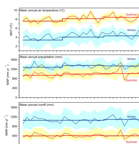
Figure 2.Mean annual air temperature (MAT, top), precipitation (MAP, middle) and runoff (MAR, bottom) for basins with summer (yellow/red) and winter (blue) low-flow minima (Fig. 1). Thin lines represent the median of mean annual values of MAT, MAP and MAR. Thick lines indicate the average for each of the three peri-ods: 1976–1986, 1987–1997 and 1998–2008. Scatter (i.e. 75 % and 25 % percentiles) indicates the variability between the basins.

overall sample size is small. Hence, the difference between both measures of effect size will be negligible for designs with large dfE, as is the case for our study. In our assessment,

measure of effect size at each catchment. A spatial synthe-sis of uncertainty contributions for basins with summer and winter low-flow regime is finally obtained from the distribu-tion of variance components across basins falling into each low-flow regime group.

3 Data

The study region is Austria (Fig. 1). Austria represents the diverse climate and physiographic conditions of central Eu-rope, which are reflected in different hydrologic regimes (Gaál et al., 2012). The topography varies from 115 m a.s.l. in the lowlands to more than 3700 m a.s.l. in the Alps. Aus-tria is located in a temperate climate zone influenced by the Atlantic, meridional south circulation and the continen-tal weather systems of Europe. Mean annual air temperature varies between−8 to 10◦_{C. The mean annual precipitation}

ranges from 550 mm yr−1 in the Danube lowlands, to more than 3000 mm yr−1on the windward slopes of the Alps.

The analysis is based on daily river flow measurements at 262 gauges (Fig. 1). This data set represents a subset of data used in Laaha and Blöschl (2006), which consists of gauges for which hydrographs are not seriously affected by abstractions and karst effects during the low-flow peri-ods. Figure 1 shows two main low-flow regimes in Austria; yellow circles indicate 130 stations with dominant summer (June–November) low-flow occurrence and blue circles in-dicate 132 gauges with winter (December–May) flow min-ima. These two groups represent basins with distinct low-flow seasons, which are controlled by different hydrologic processes. While the winter flow minima in the mountains are controlled by freezing processes and snow storage, sum-mer low flows occur during long-term persistent dry periods when evapotranspiration exceeds precipitation. The differ-ent low-flow generating processes, together with the hydro-climatic variety of the study area, gives rise to an enormous spatial complexity of low flows in Austria. The largest val-ues occur in the Alps, with typical valval-ues ranging from 6 to 20 l s−1km−2. The lowest values occur in the east rang-ing from 0.02 to 8 l s−1km−2, although the spatial pattern is much more intricate.

Climate data used in hydrologic modelling consists of mean daily precipitation and air temperature measurements at 1091 and 212 climate stations in the period 1976–2008. Model inputs have been prepared by spatial interpolation and zonal averaging described in detail in previous modelling studies (please see e.g. Merz et al., 2011 or Parajka et al., 2007). These data serve as a basis for hydrologic model cal-ibration and as a reference for future change simulations. Figure 2 shows basin averages of mean annual air temper-ature, precipitation and runoff in the period 1976–2008. The two groups of basins (winter vs. summer low-flow regimes) clearly differ in the climate regime. Basins with summer low flows are characterised by higher air temperatures, less

0.5 0.6 0.7 0.8 0.9 1.0

Runoff efficiency Z

Q

(-)

0.0 0.2 0.4 0.6 0.8 1.0

Weight wQ (-)

cal. 1976–86 cal. 1987–97 cal. 1998–08

0.0 0.2 0.4 0.6 0.8 1.0

Weight wQ (-)

0.0 0.2 0.4 0.6 0.8 1.0

Weight wQ (-)

Winter Summer

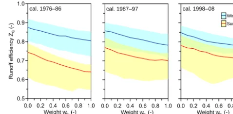
Figure 3.Runoff model efficiency (ZQ) for different calibration

weightswQin three different calibration periods. Lines represent

the medians, scatter (i.e. 75–25 % percentiles) shows theZQ

vari-ability over basins with dominant winter (blue) and summer (or-ange) low-flow regime.

precipitation and less runoff. The comparison of 3 different decades indicates that mean annual air temperatures have in-creased by 1◦C in the period 1976–2008. This increase is similar for both groups of basins. Interestingly, the mean annual precipitation has increased over the last 3 decades, which is likely compensated by increased evapotranspiration, as the mean annual runoff remains rather constant.

The RCM scenarios used in this study are based on the results of the reclip.century project (Loibl et al., 2011). The ensemble climate projections are represented by COSMO-CLM RCM runs forced by the ECHAM5 and HADCM3 global circulation models for three different Intergovern-mental Panel on Climate Change (IPCC) emission scenarios (A1B, B1 and A2; Nakicenovic et al., 2000). These represent a large spread of different emission pathways from a “busi-ness as usual” scenario with prolonged greenhouse gas emis-sions (A2), a scenario with moderate decline of emisemis-sions after 2050 (A1B) and a scenario indicating considerably re-duced emissions from the present onwards (B1).

Table 2 summarises the annual and seasonal differences (delta changes) of mean basin precipitation and air temper-ature between the future (2021–2050) and reference (1978– 2007) periods. Table 2 indicates that the largest warming is obtained by simulations driven by HADCM3. The median of air temperature increase in summer exceeds 2◦_{C. In}

Table 2.Summary of seasonal and annual changes in the mean basin precipitation and air temperature as simulated by four selected RCM runs. The first value and values in the brackets are the median and range (min/max) of differences between the future (2021–2050) and reference (1978–2007) periods in 262 basins. Winter and summer seasons are defined as December–May and June–November, respectively.

Delta change WEGC∗ECHAM5 A1B ZAMG∗∗ECHAM5 A2 AIT∗∗∗HADCM3 A1B ZAMG ECHAM5 B1

Air temperature

winter (◦C) +1.5 (0.9/1.7) +0.7 (−1.1/2.1) +1.3 (0.8/1.5) +1.0 (−0.8/2.5)

Air temperature

summer (◦C) +1.2 (0.8/1.7) +0.9 (−0.1/2.2) +2.1 (1.4/2.4) +1.3 (0.4/2.5)

Air temperature

year (◦C) +1.3 (0.9/1.5) +0.8 (−0.4/2.2) +1.7 (1.2/1.9) +1.2 (0.0/2.5)

Precipitation

winter (%) +8.2 (−0.7/16.2) −1.5 (−5.8/6.4) +1.3 (−9.6/6.8) 0.0 (−8.5/3.3)

Precipitation

summer (%) −6.2 (−9.9/3.7) +0.2 (−8.9/5.7) −5.0 (−13.5/0.2) −2.3 (−6.3/2.5)

Precipitation

year (%) +0.9 (−4.6/8.7) −0.9 (−4.1/3.4) −2.0 (−9.3/1.8) −1.2 (−5.5/2.8)

∗_{WEGC=Wegener Center for Climate and Global Change} ∗∗_{ZAMG=Zentralanstalt für Meteorologie und Geodynamik} ∗∗∗_{AIT=Austrian Institute of Technology}

-90 -60 -30 0 30 60 90

SIsim

-SI

obs

(days)

0.0 0.2 0.4 0.6 0.8 1.0

Weight wQ (-)

0.0 0.2 0.4 0.6 0.8 1.0

Weight wQ (-)

0.0 0.2 0.4 0.6 0.8 1.0

Weight wQ (-)

-50 -25 0 25 50

(Q95

sim

-Q95

obs

) / Q95

obs

(%)

0.0 0.2 0.4 0.6 0.8 1.0

cal. 1976–86 cal. 1987–97 cal. 1998–08

0.0 0.2 0.4 0.6 0.8 1.0 0.0 0.2 0.4 0.6 0.8 1.0

Winter Summer

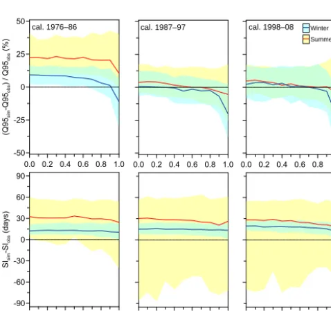
Figure 4. Difference between simulated and observed low-flow

characteristics (top panels low-flow quantile Q95, bottom panels

seasonality index SI) for different calibration variants (wQ) and

cal-ibration periods. Lines represent the median, scatter (i.e. 75–25 % percentiles) show the variability over basins with dominant winter (blue) and summer (orange) low-flow regime. The differences are estimated between model simulations and observations in the entire reference period 1976–2008.

4 Results

4.1 Low-flow simulations and uncertainty in the reference period

The runoff model efficiency (ZQ) in the three calibration pe-riods obtained for different variants of the objective function is presented in Fig. 3. The results show that ZQ is larger and thus runoff simulations are more accurate in basins with winter (blue colour) than summer low-flow minimum (red colour). Most of the basins with a winter low-flow regime are situated in the alpine western and central part of Austria, where the runoff regime is snow dominated. Such a regime has stronger runoff seasonality (see e.g. Fig. 5 in Laaha et al., 2015) and less difference in rainfall regime, which al-lows one to model the rainfall–runoff process easier than in basins with rainfall-dominated runoff regime.ZQincreases with decreasing weightwQ, which indicates that the runoff model performance likely tends to be better for low than high flows. The comparison ofZQ in the three calibration peri-ods indicates that the difference in model performance be-tween basins with winter and summer low-flow regime is the largest in the period 1976–1986. WhileZQfor basins with winter low-flow regime is very similar in all three calibra-tion periods,ZQhas an increasing tendency in basins with summer low-flow regime. For example, the median ofZQ forwQ=1.0 increases from 0.64 in the period 1976–1986 to 0.71 in the period 1998–2008. This increase is likely re-lated to the increasing number of climate stations and data quality (Merz et al., 2009).

How the different calibration variants and periods trans-late into low-flow 95 %-quantileQ95 and seasonality SI is

pe-1992 1993 1994 1995 0

2 4 6 8

Discharge

(m

3 s )

80 60 40 20 0

Precipitation (mm day )

–1

–1

Figure 5.Comparison of observed (blue) and simulated (red) flow for Hoheneich/Braunaubach, 291.5 km2). Thick lines show flows below

low-flow quantile Q95. Model simulations are based on calibration variantwQ=0.5 in the period 1998–2008. The relative difference

betweenQ95estimated from simulated and observed flows is 8 %.

wQ=0.5, 3 cal. periods

wQ=0.0, 3 cal. periods

cal.1976–86, 11 cal. variants

cal.1998–08, 11 cal. variants

0–10 % 10–20 % 20–30 % 30–40 % 40–60 % 60 % and more

Figure 6.Uncertainty ofQ95 model simulations estimated from 11 calibration variants calibrated in the same calibration period (right

panels: top – calibration period 1976–1986, bottom – calibration period 1998–2008) and from three calibration periods calibrated by the

same calibration variant (left panels: topwQ=0.5, bottomwQ=0.0). The uncertainty is expressed as the range of relative differences (%)

between simulated and observedQ95obtained by particular calibration variants in the period 1976–2008. Colour patterns in the background

show the interpolated ranges by using top-kriging method (Skoien et al., 2014; Parajka et al., 2015).

riod 1976–2008. The results show that the model calibrated in the period 1976–1986 significantly overestimatesQ95of

the reference period particularly in basins with summer low-flow regime. The period 1976–1986 is characterised by lower air temperatures with less evapotranspiration and relatively higher runoff generation rates, which translates into differ-ent soil moisture storage (FC model parameter) and runoff generation (BETA) model parameters. Such effects are con-sistent with findings of Merz et al., (2011). The hydrologic model applied to the entire reference period hence produces larger runoff contribution, which tends to overestimateQ95

particularly in the warmer and drier parts of the reference pe-riod and drier and warmer parts of Austria. The overestima-tion is consistent for large range ofwQ(wQin the range 0.0– 0.9) and the median of Q95 difference exceeds 20 %. Also

the scatter around the median is rather large, where 25 % of the basins with the summer low-flow regime have Q95

dif-ferences larger than 35 %. The simulatedQ95in basins with

winter low flows fit closer to the observed estimates. The median is less than 10 % for variants wQ< 1. Interestingly,

the model simulations based on calibration periods 1987– 1997 and 1998–2008 are much closer to the observed val-ues. The results for both groups of basins are very similar and essentially unbiased in terms of 95 % low-flow quantile. The exception is the calibration variant wQ=1 that tends to underestimateQ95. There are many significant differences

between calibration to low-flow only (wQ=0.0) and other weights, with the exception ofwQ=1, which represents a typical calibration of using classical Nash–Sutcliffe coeffi-cient.

wQ=0.5, 3 cal. periods

wQ=0.0, 3 cal. periods

cal. 1976–86, 11 cal. variants

cal. 1998–08, 11 cal. variants

0–7 7–14 14–30 30–90

90 and more (days)

Figure 7.Uncertainty of simulations of low-flow seasonality (SI) estimated from 11 calibration variants calibrated in the same calibration period (right panels: top – calibration period 1976–1986, bottom – calibration period 1998–2008) and from three calibration periods calibrated

by the same calibration variant (left panels: topwQ=0.5, bottomwQ=0.0). The uncertainty is expressed as the range of differences (days)

between simulated and observed SI in the period 1976–2008. Colour patterns in the background show the interpolated ranges by using top-kriging.

season of low-flow occurrence with more than 2 months shift (earlier or later) in almost 50 % of the basins. A typical exam-ple of such shift is provided in Fig. 5. The periods with flows below 95 % quantile are often very short and the timing of simulated low flows does not fit well with these periods. In some cases there is also a difference in the length of observed and simulated low-flow periods. Some small rainfall–runoff events in the summer or autumn cause an interruption of the observed low-flow periods, but the model simulates a com-plete absorption of the precipitation event by the soil storage and hence a longer low-flow period.

The spatial pattern of the variability ofQ95 estimation in

the reference period 1976–2008 is presented in Fig. 6. Fig-ure 6 shows the range of differences between simulated and observedQ95 for the different calibration variants. The

re-sults indicate that theQ95differences vary more between the

different objective functions (right panels); however, in many basins the range exceeds 60 % even if the model is calibrated by one objective function but in the different calibration peri-ods. As already indicated in Fig. 4, the differences are larger in basins with summer low flows, particularly for variants calibrated in the period 1976–1986. For particular basins, the differences are not strongly related to the weightwQused in the calibration, with an exception ofwQ=1, which tends to have the largest difference to observedQ95. Some examples

of the model performance for individual basins are given in the companion paper by Laaha et al. (2015).

Spatial variability of the model variability in terms of low-flow seasonality is presented in Fig. 7. The results clearly indicate that basins with winter low-flow regime (i.e. situ-ated in the Alps) vary significantly less for different calibra-tion settings than the basins with summer low-flow regime.

The range of differences is typically less than 14 days in the mountains, compared to more than 90 days in many basins with the summer low-flow regime.

The comparison of SI andQ95 ranges indicates that large

SI variability does not systematically mean large variability in terms ofQ95. For example, a cluster of basins situated

in the south-eastern part of Austria (Styria) has a large SI range of difference (i.e. more than 90 days) for 11 calibration variants in the period 1976–1986, but the variability inQ95is

in many basins less than 20 % for this case. The same applies for the opposite case of small SI and largeQ95variability in

the alpine basins.

4.2 Low-flow projections and uncertainty in the future period

Low-flow projections for selected climate scenarios and dif-ferent calibration weightswQare presented in Fig. 8. Rather than to evaluate in detail the projections in terms of abso-lute values of low-flow changes, the main focus is to assess the range of possible changes caused by different scenarios and objective function used for model calibration. The re-sults show projections based on model calibration in 1998– 2008, but the results are almost identical with results for the other two calibration periods (i.e. the average difference is around 1 %). Figure 8 clearly shows the difference in pro-jections for basins with summer and winter low-flow regime, particularly forQ95 changes. It is hence important to

decreas--50 -25 0 25 50

95

(%)

Winter

Summer

-30 -20 -10 0 10 20 30

0.0 0.2 0.4 0.6 0.8 1.0 Weight wQ (-)

ZAMG_ECHAM5_B1 AIT_HADCM3_A1B

ZAMG_ECHAM5_A2 WEGC_ECHAM5_A1B

0.0 0.2 0.4 0.6 0.8 1.0 Weight wQ (-)

0.0 0.2 0.4 0.6 0.8 1.0 Weight wQ (-)

0.0 0.2 0.4 0.6 0.8 1.0 Weight wQ (-)

Earlier

Later

Figure 8.Projections of low flows for selected climate scenarios and calibration variants. Line represents the medians, scatter (i.e. 75–25 %

percentiles) shows the variability over 262 basins. Top and bottom panels show projected changes of low-flow quantilesQ95and seasonality

index SI in basins with winter (blue) and summer (orange) low-flow regimes, respectively. Projections indicate future changes with respect to the reference period 1976–2008. Calibration variants are calibrated in the period 1998–2008.

WEGC_ECHAM5_A1B

AIT_HADCM3_A1B

ZAMG_ECHAM5_A2

ZAMG_ECHAM5_B1

-40 % and less -40 to -20 % -20 to -5 % -5–5 %

5–20 % 20–40 % 40 % and more

Figure 9.Projections of low-flow quantilesQ95 changes for four climate scenarios in 262 Austrian basins. Model simulations are based

on variant wQ=0.5 calibrated in the period 1998–2008. Colour patterns in the background show the interpolated projections by using

top-kriging.

ing low flows in the summer period. The increase of winter

Q95slightly varies between climate scenarios and tends to

in-crease for calibration variants with largerwQ. The difference in median betweenwQ< 0.4 andwQ> 0.8 is approximately 9 %. The projections ofQ95changes in basins with summer

low flows have significantly smaller variability and do not depend onwQ. The change in low-flow seasonality (Fig. 8, bottom panels) is less pronounced. The median of projections

is around 5 and 10 days earlier than in the reference period for basins with summer and winter low-flow regime, respec-tively. Interestingly, the variability between basins andwQis significantly smaller than that obtained for different calibra-tion variants in the reference period (Fig. 4).

Examples of spatial patterns of low-flow projections are presented in Figs. 9 and 10. The projections ofQ95changes

typ-WEGC_ECHAM5_A1B

AIT_HADCM3_A1B

ZAMG_ECHAM5_A2

ZAMG_ECHAM5_B1

less than 90 days (earlier) -90 to -30 days -30 to -7 days 7 to -7 days 7–30 days 30–90 days

more than 90 days (later)

Figure 10.Projections of changes in low-flow seasonality (SI) for four climate scenarios in 262 Austrian basins. Model simulations are

based on variantwQ=0.5 calibrated in the period 1998–2008. Colour patterns in the background show the interpolated projections by using

top-kriging.

WEGC_ECHAM5_A1B

AIT_HADCM3_A1B

ZAMG_ECHAM5_A2

ZAMG_ECHAM5_B1

0–10 % 10–20 % 20–30 % 30–40 % 40–60 % 60 % and more

Figure 11.Uncertainty ofQ₉₅model projections of low flows for four different climate scenarios. The uncertainty is expressed as the range

of relative differences (%) betweenQ95simulated in the future and reference period obtained for 11 calibration variants calibrated in three

calibration periods. Colour patterns in the background show the interpolated ranges by using top-kriging.

ically in the range of 10–30 %. A decrease is simulated in south-eastern part of Austria (Styria) mostly in the range of

−5 – (−20) %. The most spatially different projection is pro-vided by the HADCM3 A1B climate scenario, which sim-ulates the strongest gradient between an increase of Q95 in

the Alps in winter and a decrease in the south-eastern region in summer. The change in the seasonality varies between the scenarios, but there is a tendency for earlier low flows in the northern Alps and a shift to later occurrence of low flows in eastern Austria (Fig. 10). As already indicated in Fig. 8, the shift in seasonality is greater than 1 month only in a few basins.

Figures 9 and 10 show projections of low flows for four climate scenarios, but only one set of hydrologic model

pa-rameters. The evaluation of the impacts of different calibra-tion variants on the variability of low-flow projeccalibra-tions is pre-sented in Figs. 11 and 12. These figures indicate the range of Q95 (Fig. 11) and the seasonality occurrence (Fig. 12)

changes obtained by 11 calibration variants and 3 calibration periods. The range ofQ95changes is interestingly the largest

in basins with the winter low-flow regime. In the Alps, the increase ofQ95 is often in the range of 15 % to more than

60 %. On the other hand, the futureQ95 estimates vary only

WEGC_ECHAM5_A1B

AIT_HADCM3_A1B

ZAMG_ECHAM5_A2

ZAMG_ECHAM5_B1

0–7 7–14 14–30 30–90 90 and more (days)

Figure 12.Uncertainty of model projections of low-flow seasonality for four different climate scenarios. The uncertainty is expressed as the range of relative differences (%) between seasonality occurrence (SI) simulated in the future and reference period obtained for 11 calibration variants calibrated in three calibration periods. Colour patterns in the background show the interpolated ranges by using top-kriging.

0–10 % 10–20 % 20–30 % 30–40 % 40–60 % 60 % and more

0–7 7–14 14–30 30–90 90–150 150 and more

0.0–0.2 0.2–0.4 0.4–0.6 0.6–0.8 0.8–1.0 1.0 and more

0.0–0.5 0.5–1.0 1.0–2.0 2.0–3.0 3.0–4.0 4 and more

Total range: Q95 projections (%) Total range: SI projections (days)

Range projections / Range calibrations Range projections / Range calibrations

Figure 13.Total uncertainty of model projections of low flows for four different climate scenarios, 11 calibration variants and three calibration

periods. The uncertainty is expressed as the range ofQ95(left panel) and seasonality (right panel) of differences between model simulations

in the future and reference periods. Bottom panels show the ratio between the range of climate projections to the range of differences in the reference period. Colour patterns in the background show the interpolated ranges by using top-kriging.

seasonality can vary within more than 3 months, e.g. in the south-eastern part of Austria.

The total uncertainty of low-flow projections of Q95 and

SI is presented in Fig. 13. While the top panels show the range of low-flow characteristics for all climate scenarios, calibration variants and periods, the bottom panels show the ratio between the uncertainty of future low-flow projections to the range of low-flow indices simulated in the reference period. The results show that theQ95range is less than 25 %

in approximately one-third of analysed basins. On the other hand, 20 % of basins have a range larger than 50 %. These are the basins with the winter low-flow regime. The

variabil-ity in the date of low-flow occurrence is less than 3 months in 40 % of the basins. In almost 20 % of the basins, how-ever, it is larger than 5 months. The ratio between the range of projections to the range of calibration differences (bottom panels in Figs. 13 and 14) indicates that only in 15 % of the cases is the climate projection uncertainty ofQ95larger than

the range obtained in the calibration period. Most of these basins are situated in the mountains (mean basin elevation above 1000 m a.s.l.) and have winter low-flow regime. The range of calibratedQ95is larger in almost all basins with the

an-Projection unc. larger

Calibration unc. larger

Projection unc. larger

Calibration unc. larger

0.0 0.4 0.8 1.2 1.6 2.0

Q95

projection/calibration uncertainty ratio (-)

Projection unc. larger

Calibration unc. larger

0 0.4 0.8 1.2 1.6 Aridity index (-)

Projection unc. larger

Calibration unc. larger

0 1000 2000 3000 Mean basin elevation (m a.s.l.)

Projection unc. larger

Calibration unc. larger

10 100 1000 10000 Basin area (km2)

0.0 0.1 1.0 10.0 100.0

SI projection/calibration uncertainty ratio (-)

Projection unc. larger

Calibration unc. larger

Figure 14.Relationship between the uncertainty ratio between calibration and projection uncertainty and basin area (left panels), mean basin

elevation (middle panels) and aridity index (right panels). Top and bottom panels show the uncertainty ratio for the low-flow quantile (Q95)

and seasonality index (SI), respectively. Basins with winter low-flow seasonality are plotted in blue, basins with summer low-flow seasonality are in yellow.

0 20 40 60 80 100

Uncertainty contribution (%)

Climate scenario

Calibration decade

Calibration obj. function

Residuals _Climate

scenario Calibrationdecade obj. functionCalibration Residuals

Winter Summer

Figure 15.Relative contribution of the three variance components (i.e. climate scenario, calibration decade and objective function) to the overall uncertainty of future low-flow projection in basins with winter (left panel) and summer (right panel) low-flow regime. The boxes and whiskers show 25 and 75 % percentiles and 5 and 95 % percentiles of the uncertainty contributions in 130 (summer low-flow regime) and 132 (winter low-flow regime) basins, respectively.

nual potential evaporation to mean annual precipitation). On the other hand, the climate projection uncertainty dominates for the low-flow seasonality and is more than 3 times larger in 50 % of basins, particularly in the Alps. The SI projection uncertainty is only in 15 % of the basins lower than the SI range obtained in the calibration period. The SI uncertainty ratio tends to be lower with increasing mean basin elevation and the basin area, but there is no apparent relationship with the aridity of the basins.

The relative contribution of the three main variance com-ponents (i.e. climate scenario, decade used for model calibra-tion and calibracalibra-tion variant representing different objective

the median contribution from climate scenario is larger than 76 %.

5 Discussion and conclusions

The objective of the study is to explore the relative role of hydrologic model calibration and climate scenarios in the un-certainty of low-flow projections. While many previous stud-ies simulate only the change in hydrologic regime or extreme characteristics due to changes in climate, in this study we fo-cus on the quantification of the range of low-flow projections (i.e. uncertainty) due to differences in the objective function used in model calibration, temporal stability of model param-eters and an ensemble of climate projections.

There are a number of studies that compare the uncertainty of projected runoff changes due to different model structure, objective function or GCM and emission scenarios. These studies found that the hydrologic model uncertainty tends to be considerably smaller than that from GCM or emission sce-narios (Najafi et al., 2011; Prudhomme and Davies, 2009). Such results, however, refer to the seasonal or monthly runoff and are based on only a limited number of basins. The quan-tification of the uncertainty in low flows is still rather rare. Some studies (e.g. Huang et al., 2013; Forzieri et al., 2014) evaluate the low-flow uncertainty in terms of the number of projections with the same change direction. They showed that the uncertainty is controlled mainly by the differences in emission scenarios and it decreases with increasing pro-jection horizon. Our results indicate that, although the uncer-tainty from different climate scenarios is larger than 40 % in many basins, the range of low-flow indices from model cal-ibration can exceed 60 %. This result particularly relates to the assessment of low-flow quantile changes.

Some recent low-flow studies suggest to more explicitly distinguish between the processes leading to low-flow situa-tions (see e.g. Fleig et al., 2006; Laaha et al., 2006; Van Loon et al., 2015; Forzieri et al., 2014). Following this recommen-dation, we analysed the effects of model calibration and cli-mate scenarios separately for basins with dominant winter and summer low-flow regimes. Our results indicate that the calibration runoff efficiency in basins with winter low-flow regime is larger (more accurate), and varies between basins less than in basins with summer low-flow regime. The cal-ibration uncertainty in basins with summer low flows ex-ceeds in many basins 60 % even if the model is calibrated by the same objective function but in different calibration pe-riods. This finding confirms and quantifies the potential im-pact of time stability of model parameters reported by Merz et al. (2011). The model parameters calibrated in colder pe-riods with relatively larger runoff generation rates tend to overestimate low flows, particularly in basins with a summer low-flow regime and in warmer and drier parts of the sim-ulation period. The results indicate that the time stability of model parameters is not sensitive to the weighting of normal

(ME) and logarithmic transformed (M_Elog) Nash–Sutcliffe

ef-ficiency in the objective function used for calibration. The exception is the case of using onlyME with no weight on M_Elog, which does not allow for accurate low-flow simula-tions. This finding partly supports the studies that propose logarithmically transformed discharge values for calibrating hydrologic models with a focus on low flows (please see re-view in Pushpalatha et al., 2012). Our results show that the impact of the objective function is larger for SI estimation in basins with summer low-flow regime in the reference pe-riod and for future projections ofQ95 in basins with winter

low-flow regime. Depending on the calibration variant, the change in seasonality can vary within more than 3 months, which clearly indicates a shift in the main hydrologic pro-cesses causing the low flows.

The climate change signals captured in selected scenarios are well within the range of the projections of the ENSEM-BLES regional climate simulations for Europe (Van der Lin-den and Mitchell, 2009; Heinrich and Gobiet, 2011). Jacob et al. (2014) showed that the most recent regional climate simu-lations over Europe, accomplished by the EURO-CORDEX initiative (Moss et al., 2010), are rather similar to the older ENSEMBLES simulations with respect to the climate change signal and the spatial patterns of change. Although this en-semble of four scenario runs seems rather small, the selection accomplished by the reclip:century consortium was not arbi-trary, but based on quantitative metrics. Prein et al. (2011) in-vestigated the performance of all GCMs in CMIP3 for central Europe based on a performance index including various pa-rameters. They found that for the given domain the ECHAM5 and the HADCM3 showed the highest scores, which justi-fied the selection of these GCMs for driving the RCM. In addition, these two models show different climate sensitiv-ity, where the warming over the course of the 21st century is lower in ECHAM5 and higher in HADCM3. This fea-ture in combination with the utilisation of three different scenarios for ECHAM5 provides broad ensemble bounds, although the climate change signal of the different scenar-ios for the given investigation period (2021–2050) is rather similar, particularly for air temperature (cf. Table 1). The projected future decrease ofQ95 is most pronounced in the

AIT_HADCM3_A1B run, particularly in basins with sum-mer low-flow regime in the low lands. As indicated in Hein-rich and Gobiet (2011), the climate sensitivity of HADCM3 is higher than that of ECHAM5, which translates into a higher warming rate of 2.1◦C in summer (cf. Table 1) com-pared to 1.2◦C in the ECHAM5-driven run. The higher evap-orative demand due to the increased air temperature signal translates into the strongest change of the summer low-flow signal.

of low-flow magnitudes is larger for simulations in the refer-ence period, while the range of seasonality is larger for future projections. Previous ENSEMBLES and CORDEX studies showed that RCM uncertainty is far from being negligible for hydrology-related variables. Even if only one RCM is tested here and the variability and uncertainty of GCM and emission scenarios can be large, the results clearly indicate the importance of selecting objective functions in hydrologic model calibration for simulating low-flow projections.

In our study, we use a three-way ANOVA approach to decompose the contribution of climate scenarios and hy-drologic model settings to the total uncertainty of low-flow projections. While previous studies (e.g. Hingray and Said, 2014; Lafaysse et al., 2014; Vidal et al., 2015) assessed the variance components of a temporal change from the multi-member ensemble runs in individual basins, in our study, we lumped the temporal change to one time slice (future hori-zon) and assessed the variance components in a spatial con-text of 262 basins. The spatial synthesis of the uncertainty contribution is evaluated for two groups of basins, repre-senting two main (summer and winter) low-flow regimes in Austria. We found that the relative contribution of three vari-ance components – climate scenarios, calibration decade and calibration objective function differs for basins with differ-ent low-flow regimes. The uncertainty from climate scenar-ios dominates in basins with summer low flows; however, in basins with winter low flows the relative contribution from hydrological modelling is significantly larger. This is consis-tent with previous studies that show a substantial uncertainty contribution of hydrological models in basins dominated by snow- and ice melt (Addor et al., 2014; Vidal et al., 2015).

The assessment in Austria enabled us to account for one conceptual hydrologic model and two different low-flow regimes. In the future we plan to extend such comparative assessment to more types of low flows (e.g. as classified in Van Loon and Van Lanen, 2012), their combinations linked with changes in land use and management at the wider, Eu-ropean scale, as well as to account for hydrologic models of different complexity, wider range of climate scenarios and different downscaling techniques. This will allow us to shed more light on the factors controlling the possible scenarios of low-flow and water resource changes in the future.

From a practical point of view, the projections of Q95

changes and related uncertainties are an essential input to water quality modelling. The exceedance of environmen-tal quality standards (BGBl II No. 99/2010, 2010; Zessner, 2008) in case of emissions from point sources (e.g. waste water treatment plants) increases the vulnerability of water resources, particularly during low-flow conditions. We there-fore also plan to evaluate the impact of climate projection and hydrologic model uncertainties on the assessment of wa-ter quality and its changes.

Acknowledgements. We would like to thank the Austrian

Cli-mate and Energy Fund (Project B060362-CILFAD, Project no. R13AC6K11034-AQUASTRESS) and the Austrian Science Foundation (FWF Project no. P 23723-N21) for financial support. At the same time, we would like to thank the Hydrographical Service of Austria (HZB) and the Central Institute for Meteorology and Geodynamics (ZAMG) for providing hydrologic and climate data.

Edited by: J.-P. Vidal

References

Addor, N., Rössler, O., Köplin, N., Huss, M., Weingartner, R., and Seibert, J.: Robust changes and sources of uncertainty in the pro-jected hydrological regimes of Swiss catchments, Water Resour. Res., 50, 7541–7562, doi:10.1002/2014WR015549, 2014. BGBl II Nr. 99/2010: Bundesgesetzblatt für die Republik

Öster-reich, Qualitätszielverordnung Ökologie Oberflächengewässer – QZV Ökologie OG, Jahrgang 2010.

Bosshard, T., Carambia, M., Goergen, K., Kotlarski, S., Krahe, P., Zappa, M., and Schär, C.: Quantifying uncertainty sources in an ensemble of hydrological climate-impact projections, Water Re-sour. Res., 49, 1523–1536, doi:10.1029/2011WR011533, 2013. Burn, D. H.: Catchment similarity for regional flood frequency

anal-ysis using seasonality measures, J. Hydrol., 202, 212–230, 1997. Ceola, S., Arheimer, B., Baratti, E., Blöschl, G., Capell, R., Castel-larin, A., Freer, J., Han, D., Hrachowitz, M., Hundecha, Y., Hut-ton, C., Lindström, G., Montanari, A., Nijzink, R., Parajka, J., Toth, E., Viglione, A., and Wagener, T.: Virtual laboratories: new opportunities for collaborative water science, Hydrol. Earth Syst. Sci., 19, 2101–2117, doi:10.5194/hess-19-2101-2015, 2015. Chauveau, M., Chazot, S., Perrin, C., Bourgin, P., Sauquet, E.,

Vi-dal, J., Rouchy, N., Martin, E., David, J., Norotte, T., Maugis, P., and de Lacaze, X.: What impacts of climate change on sur-face hydrology in France by 2070?, La Houille Blanche, 4, 5–15, 2013.

Chiew, F. H. S., Zheng, H., and Vaze, J.: Implication of calibra-tion period on modelling climate change impact on future runoff, Proc. IAHS, 371, 3–6, doi:10.5194/piahs-371-3-2015, 2015. Coron, L., Andréassian, V., Perrin, C., Lerat, J., Vaze, J.,

Bourqui, M., and Hendrickx, F.: Crash testing hydrological models in contrasted climate conditions: An experiment on 216 Australian catchments, Water Resour. Res., 48, W05552, doi:10.1029/2011WR011721, 2012.

Dams, J., Nossent, J., Senbeta, T. B., Willems, P., and Bate-laan, O.: Multi-model approach to assess the impact of cli-mate change on runoff, Journal of Hydrology, 529(3),1601–1616 doi:10.1016/j.jhydrol.2015.08.023, 2015.

Dobler, C., Hagemann, S., Wilby, R. L., and Stötter, J.: Quantify-ing different sources of uncertainty in hydrological projections in an Alpine watershed, Hydrol. Earth Syst. Sci., 16, 4343–4360, doi:10.5194/hess-16-4343-2012, 2012.

Feyen, L. and Dankers, R.: Impact of global warming on stream-flow drought in Europe, J. Geophys. Res., 114, D17116, doi:10.1029/2008JD011438, 2009.

Finger, D., Heinrich, G., Gobiet, A., and Bauder, A.: Projections of future water resources and their uncertainty in a glacierized catchment in the Swiss Alps and the subsequent effects on hy-dropower production during the 21st century, Water Resour. Res., 48, W02521, doi:10.1029/2011WR010733, 2012.

Fleig, A. K., Tallaksen, L. M., Hisdal, H., and Demuth, S.: A global evaluation of streamflow drought characteristics, Hydrol. Earth Syst. Sci., 10, 535–552, doi:10.5194/hess-10-535-2006, 2006. Forzieri, G., Feyen, L., Rojas, R., Flörke, M., Wimmer, F.,

and Bianchi, A.: Ensemble projections of future streamflow droughts in Europe, Hydrol. Earth Syst. Sci., 18, 85–108, doi:10.5194/hess-18-85-2014, 2014.

Gaál, L., Szolgay, J., Kohnová, S., Parajka, J., Merz, R., Viglione, A., and Blöschl, G.: Flood timescales: Understand-ing the interplay of climate and catchment processes through comparative hydrology, Water Resour. Res., 48, W04511, doi:10.1029/2011WR011509, 2012.

Heinrich, G. and Gobiet, A.: reclip:century 1 Research for mate Protection: Century Climate Simulations: Expected Cli-mate Change and its Uncertainty in the Alpine Region, ACRP final report reclip:century part D, Graz, Austria, 48 pp., 2011. Hingray, B. and Said, M.: Partitioning internal variability and model

uncertainty components in a multimember multimodel ensemble of climate projections, J. Climate, 27, 6779, doi:10.1175/JCLI-D-13-00629.1, 2014.

Huang, S., Krysanova, V., and Hattermann, F. F.: Projection of low flow conditions in Germany under climate change by combining three RCMs and a regional hydrological model, Acta Geophys., 61, 151–193, 2013.

Jacob, D., Petersen, J., Eggert, B., Alias, A., Christensen, O. B., Bouwer, L., Braun, A., Colette, A., Déqué, M., Georgievski, G., Georgopoulou, E., Gobiet, A., Menut, L., Nikulin, G., Haensler, A., Hempelmann, N., Jones, C., Keuler, K., Kovats, S., Kröner, N., Kotlarski, S., Kriegsmann, A., Martin, E., Meijgaard, E., Moseley, C., Pfeifer, S., Preuschmann, S., Radermacher, C., Radtke, K., Rechid, D., Rounsevell, M., Samuelsson, P., Somot, S., Soussana, J.-F., Teichmann, C., Valentini, R., Vautard, R., Weber, B. and Yiou, P.: EURO-CORDEX: new high-resolution climate change projections for European impact research, Reg. Environ. Change, 14, 563–578, doi:10.1007/s10113-013-0499-2, 2014.

Koffler, D. and Laaha, G.: lfstat: Calculation of Low Flow Statis-tics for daily stream flow data. R package version 0.5. avail-able at: http://CRAN.R-project.org/package=lfstat (last access: 20 November 2015), 2014.

Laaha, G. and Blöschl, G.: Seasonality indices for

region-alizing low flows, Hydrolog. Process., 20, 3851–3878,

doi:10.1002/hyp.6161, 2006.

Laaha, G. and Blöschl, G.: A national low flow estimation proce-dure for Austria, Hydrol. Sci. J., 52, 625–644, 2007.

Laaha, G., Parajka, J., Viglione, A., Koffler, D., Haslinger, K., Schöner, W., Zehetgruber, J., and Blöschl, G.: A three-pillar approach to assessing climate impacts on low flows, Hydrol. Earth Syst. Sci. Discuss., 12, 13069–13122, doi:10.5194/hessd-12-13069-2015, 2015.

Lafaysse, M., Hingray, B., Mezghani, A., Gailhard, J., and Terray, L.: Internal variability and model uncertainty

com-ponents in future hydrometeorological projections: The

Alpine Durance basin, Water Resour. Res., 50, 3317–3341, doi:10.1002/2013WR014897, 2014.

Loibl, W., Formayer, H., Schöner, W., Truhetz, H., Anders, I., Go-biet, A., Heinrich, G., Köstl, M., Nadeem, I., Peters Anders, J., Schicker, I., Suklitsch, M., and Züger, H.: reclip:century 1 Research for Climate Protection: Century Climate Simulations: Models, Data and GHG Scenarios, Simulations, ACRP final re-port reclip:century part A, Vienna, 22 pp., 2011.

Merz, R., Parajka, J., and Blöschl, G.: Time stability of catchment model parameters: Implications for climate impact analyses, Water Resour. Res., 47, W02531, doi:10.1029/2010WR009505, 2011.

Moss, R. H., Edmonds, J. A., Hibbard, K. A., Manning, M. R., Rose, S. K., van Vuuren, D. P., Carter, T. R., Emori, S., Kainuma, M., Kram, T., Meehl, G. A., Mitchell, J. F. B., Nakicenovic, N., Riahi, K., Smith, S. J., Stouffer, R. J., Thomson, A. M., Weyant, J. P., and Wilbanks, T. J.: The next generation of scenarios for climate change research and assessment, Nature, 463, 747–756, 2010. Najafi, M. R., Moradkhani, H., and Jung, I. W.: Assessing the

uncer-tainties of hydrologic model selection in climate change impact studies, Hydrol. Process. 25, 2814–2826, doi:10.1002/hyp.8043, 2011.

Nakicenovic, N., Alcamo, J., Davis, G., de Vries, B., Fenhann, J., Gaffin, S., Gregory, K., Grübler, A., Jung, T. Y., Kram, T., La Rovere, E. L., Michaelis, L., Mori, S., Morita, T., Pepper, W., Pitcher, H., Price, L., Raihi, K., Roehrl, A., Rogner, H.-H., Sankovski, A., Schlesinger, M., Shukla, P., Smith, S., Swart, R., van Rooijen, S., Victor, N., and Dadi, Z.: IPCC Special Report on Emissions Scenarios, Cambridge University Press: Cambridge, UK and New York, 599 pp., 2000.

Parajka, J. and Blöschl, G.: The value of MODIS snow cover data in validating and calibrating conceptual hydrologic models, J. Hy-drol., 358, 240–258, 2008.

Parajka, J., Merz, R., and Blöschl, G.: Uncertainty and multiple objective calibration in regional water balance modelling: case study in 320 Austrian catchments, Hydrol. Process., 21, 435– 446, doi:10.1002/hyp.6253, 2007.

Parajka, J., Merz, R., Skøien, J. O., and Viglione, A.: The role of station density for predicting daily runoff by TOP-KRIGING interpolation in Austria, J. Hydrol. Hydromech., 63, 1–7, doi:10.1515/johh-2015-0024, 2015.

Prein, A. F., Gobiet, A., and Truhetz, H.: Analysis of uncertainty in large scale climate change projections over Europe, Met. Zet., 20, 383–395, 2011.

Prudhomme, Ch. and Davies, H.: Assessing uncertainties in cli-mate change impact analyses on the river flow regimes in the UK. Part 2: future climate, Clim. Change, 93, 177–195, doi:10.1007/s10584-008-9464-3, 2009.

Skoien, J.O., Blöschl, G., Laaha, G., Pebesma, E., Parajka, J., and Viglione, A.: rtop: An R package for interpolation of data with a variable spatial support, with an example from river networks, Comp. Geosci., 67, 180–190, doi:10.1016/j.cageo.2014.02.009, 2014.

re-sults from the ENSEMBLES project, Met Office Hadley Centre, Exeter, UK, 160 pp., 2009.

Van Loon, A. F. and Van Lanen, H. A. J.: A process-based typol-ogy of hydrological drought, Hydrol. Earth Syst. Sci., 16, 1915– 1946, doi:10.5194/hess-16-1915-2012, 2012.

Van Loon, A. F., Ploum, S. W., Parajka, J., Fleig, A. K., Garnier, E., Laaha, G., and Van Lanen, H. A. J.: Hydrological drought types in cold climates: quantitative analysis of causing factors and qualitative survey of impacts, Hydrol. Earth Syst. Sci., 19, 1993–2016, doi:10.5194/hess-19-1993-2015, 2015.

Vidal, J.-P., Hingray, B., Magand, C., Sauquet, E., and Ducharne, A.: Hierarchy of climate and hydrological uncertainties in tran-sient low flow projections, Hydrol. Earth Syst. Sci. Discuss., 12, 12649–12701, doi:10.5194/hessd-12-12649-2015, 2015.

Viglione, A., Parajka, J., Rogger, M., Salinas, J. L., Laaha, G., Siva-palan, M., and Blöschl, G.: Comparative assessment of predic-tions in ungauged basins – Part 3: Runoff signatures in Austria, Hydrol. Earth Syst. Sci., 17, 2263-2279, doi:10.5194/hess-17-2263-2013, 2013.

Viglione, A. and Parajka, J.: TUWmodel: Lumped Hydrological Model for Education Purposes. R package version 0.1-4. avail-able at: http://CRAN.R-project.org/package=TUWmodel, (last access: 20 November 2015), 2014.

von Storch, H. and Zwiers, F. W.: Statistical analysis in climate re-search, Cambridge University Press, Cambridge, 484 pp., 1999.

Zessner, M.: Transboundary pollution and water quality